|
Lobachevskii Journal of Mathematics Vol. 13, 2003, 3 – 13
©R. Dautov, R. Kadyrov, E. Laitinen, A. Lapin,
J. Piesk
ABSTRACT. In this paper a 3D-model for simulation and dynamic control of the continuous casting process is presented. The diffusion convection equation with multiphase transition is used as a simulation model. The developed model is discretized by finite element method and the algebraic equations are solved using pointwise relaxation method. Two different type of methods are used to control the secondary cooling, namely PID and optimal control method. The numerical results are presented and analyzed.
|
________________
Key words and phrases. Stefan problem, continuous casting process, optimization problem, FEM, implicit schemes. |
In the continuous casting process the molten steel is poured into a bottomless mold which is cooled with internal water flow. The cooling in the mold extracts heat from the molten steel and initiates the formation of the solid shell. The shell formation is essential for the support of the slab after mold exit. After the mold the slab enters into the secondary cooling area in which it is cooled by water mist sprays. The secondary cooling region is usually divided into cooling zones in which the amount of the cooling water can be controlled separately.
The control of cast cooling is of central importance in continuous casting process because it has a considerable influence on formation of cracks and other defects which can be formed in cast material. The cast should be cooled down according to a certain temperature field which depend on e.g. steel quality, cast shape, casting speed. Accurate knowledge of temperature field and liquid pool length is also important especially when using soft reduction or ”near final shape” casting. Many numerical models for simulation of the casting process have been developed in recent years [6, 9, 10]. Some of them have been applied to control and optimize casting process [4, 5, 11]. To our knowledge, all real-time industrial control applications are based on two dimensional models. In many cases two dimensional models are sufficient for control purpose. However, nowadays the highly automated and instrumented casting machines in steel factories allows the use of more sophisticated simulation and control models.
Our aim is to use the developed 3D-model in dynamic process control. We have considered PID and optimal control methods to control the secondary cooling. The two methods are very different from each other. The PID algorithm is quite simple and computationally inexpensive. However, the use of PID method is limited to the control of the surface temperature. Moreover, the PID algorithm contains experimental tuning parameters. On the other hand the optimal control method can be very complicated. The optimal control method minimizes a cost function which is constructed by means of metallurgical cooling criteria. Several different cooling criteria can be used, e.g. the maximum length for the liquid pool, the maximum reheating and cooling rates on the slab surface, the minimum and maximum temperature at the unbending point and the maximum and minimum temperature on the surface along the casting machine [6]. The development work of our optimal control model is still ongoing. Therefore we use quite simple cost function in our numerical example.
Let
where
We define the temperature
where
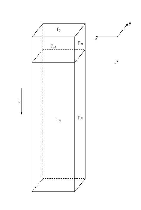
The mathematical model of the continuous casting problem can be written as:
Here
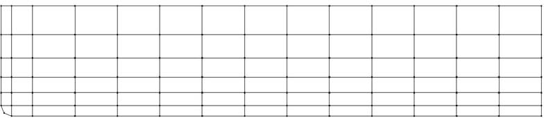
We partition
Step sizes are smaller near left and down boundaries of
We discretize our problem in time by using semi-implicit
approximation, more precisely, we approximate the term
|
| (2) |
We denote by
The weak solution of the semi-discrete problem is defined by integral identity
|
| (3) |
for all trial functions
Let
is the finite element approximation of
for every function
Approximation of the semi-discrete problem (3) by a finite element scheme is defined as
|
| (4) |
for all trial functions
|
| (5) |
where
More precisely, let
Therefore matrix
and for matrices
Temperature dependent enthalpy
We note that to implement our method it is sufficient to construct only 2D- and 1D-matrices. Therefore the computational efficiency of our model is very good. Also the memory allocation requirements are not so strong than in the case of ordinary 3D-brick elements.
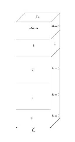
The secondary cooling region is divided into cooling zones
(see figure 3) in which the values of heat transfer coefficients,
Two different control methods are used for optimizing the secondary cooling process on the boundary of the steel slab, namely PID and optimal control method.
4.1. PID control. In PID control the water cooling in each secondary cooling zone is
done separately and indepentendly of each other. Heat transfer coefficient in each cooling
zone
|
| (6) |
where
|
| (7) |
with constant time step
4.2. Optimal control. In optimal control method our aim is to minimize
a cost function which is constructed by means of metallurgical cooling
criteria. We can formulate our optimal control problem in the following
way:
Find
|
| (8) |
where
Our cost function,
To solve the optimal control problem (8) we use the following gradient method. For given
initial guess
|
| (9) |
where
|
| (10) |
where
and
is the approximation of the cost function
and we derive a system of linear algebraic equations
|
| (11) |
After solving the adjoint state problem (11) the descent direction
is found.
Choose a
The optimal step size in the equation (9) is still unknown. We use the following algorithm to
determine
If
Else
For
If
Else
Our aim is to use the optimal control method in dynamic casting process.
At each iteration the calculation of the solution of the discretized state
problem (5) is needed, which is very time consuming. Therefore, we use
Here we present some numerical results for solving continuous casting problem. The secondary cooling region is divided into eight cooling zones. The essential input parameters are presented in the table 1.
|
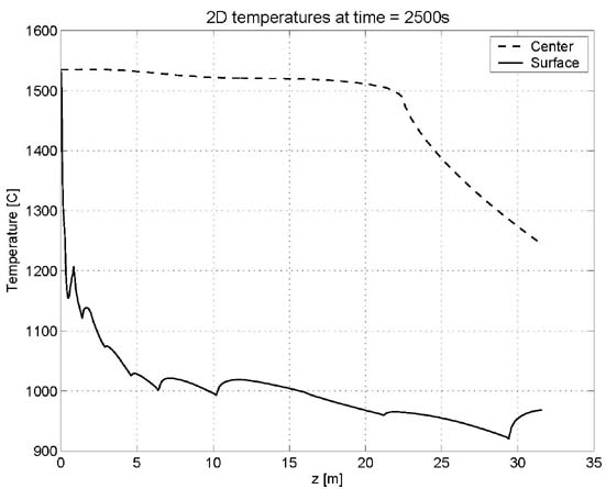
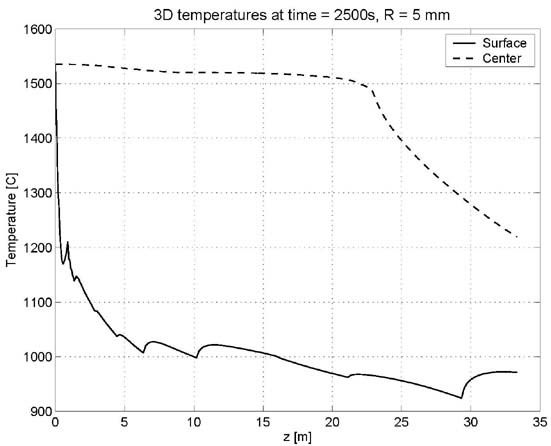
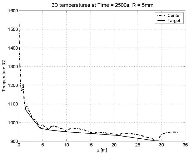
In our first numerical test we compare our 3D-model with existing
2D continuous casting model used at Rautaruukki steel factory in
Finland. The cooling is assumed to be constant along each cooling zone
during the casting process. Thus, the values of heat transfer coefficients
|
|
|
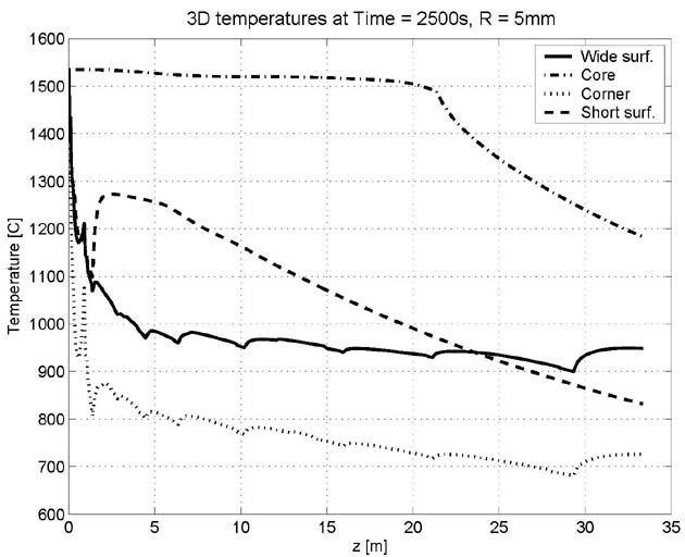
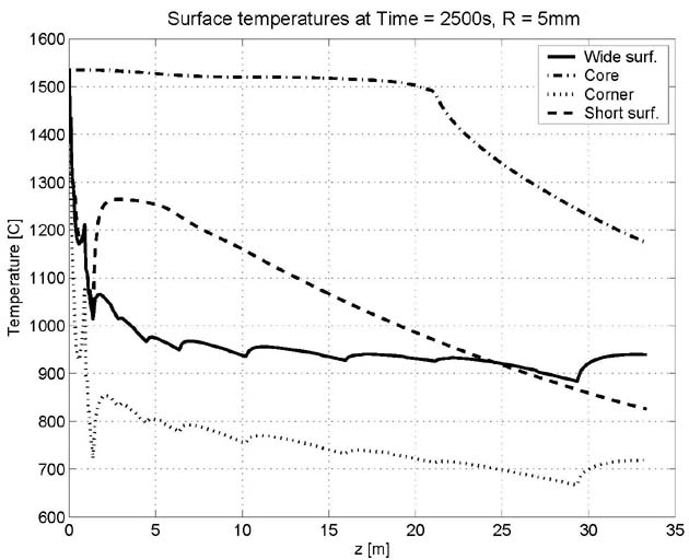
We are also interested in calculated lengths of liquid pool (longitudinal
length of the liquidus isotherm in the centre of the slab), ’stable’ liquid pool
(
|
Our results show that calculated temperature fields of the two models are very similar but a difference in calculated lengths of liquid pools appear. From the control point of view the information about temperature field and the pool lengths is important because internal cracks of final product arise during solidification process. Moreover, soft reduction technology requires exact information about liquid and mushy pool lengths.
In our second numerical test the PID and optimal control algorithms were also
tested to optimize the secondary cooling i.e. heat transfer coefficients. The results
are shown in figures 5 and 6. We can see from the figure 5 that PID control
algorithm adjusts water cooling in the way that the difference between target and
calculated temperatures at the end of each cooling zone is minimized. The
optimal control method on the other hand minimizes the cost function
|
|
[1] S. Bouhouche, Contribution to quality and process optimisation in continuous
casting using mathematical modelling, Doctoral Dissertation, der Technischen
Universit
[2] J. Jr. Douglas and T.F. Russel, Numerical methods for convection-dominated diffusion problem based on combining the method of characteristic with finite element or finite difference procedures, SIAM J. Numer. Anal., V. 19., (1982), pp. 871–885.
[3] C. M. Elliot and J. R. Ockendon, Weak and variational methods for moving boundary problems. Pitman Advanced Publishing Program, Boston, (1982).
[4] B. Filipic, B. Sarler, Evolving parameter settings for continuous casting of steel, in Proceedings of the 6th European Congress on Intelligent Techniques & Soft Computing, Aachen, Germany, (1998), pp. 444–449.
[5] M. Jauhola, E. Kivel
[6] E. Laitinen, On the simulation and control of the continuous
casting of steel, Doctoral Dissertation, University of
Jyv
[7] E. Laitinen, A. Lapin, J. Piesk
[8] E. Laitinen, J. Piesk
[9] S. Louhenkilpi, E. Laitinen, R. Nieminen, Real-time simulation of heat transfer in continuous casting, Metall. Trans., Vol. B24, (1993), pp. 685–693.
[10] J.F Rodrigues, F. Yi, On a two-phase continuous casting Stefan problem with nonlinear flux, Euro. J. App. Math., Vol. 1, (1990), pp. 259–278.
[11] C.A Santos, J.A. Spim Jr., M.C.F. Ierardi, A. Garcia, The use of artificial intelligence technique for the optimisation of process parameters used in the continuous casting of steel, Applied Math. Modelling., 26, (2002), pp. 1077–1092.
KAZAN STATE UNIVERSITY, DEPARTMENT OF APPLIED MATHEMATICS, 18, KREMLEVSKAYA ST., KAZAN, RUSSIA, 420008
E-mail address: rdautov@ksu.ru
KAZAN STATE UNIVERSITY, DEPARTMENT OF APPLIED MATHEMATICS, 18, KREMLEVSKAYA ST., KAZAN, RUSSIA, 420008
E-mail address: rkadyrov@ksu.ru
UNIVERSITY OF OULU, FINLAND.
E-mail address: ejl@sun3oulu.fi
KAZAN STATE UNIVERSITY, DEPARTMENT OF APPLIED MATHEMATICS, 18, KREMLEVSKAYA ST., KAZAN, RUSSIA, 420008
E-mail address: alapin@ksu.ru
UNIVERSITY OF OULU, FINLAND.
E-mail address: jpieska@sun3.oulu.fi
UNIVERSITY OF OULU, FINLAND.
E-mail address: valtteri@mail.student.oulu.fi
Received October 15, 2003