Lobachevskii Journal of Mathematics
Vol. 13, 2003, 25 – 38
©R.F. Kadyrov, E. Laitinen, and A.V. Lapin
R.F. Kadyrov, E. Laitinen, and A.V. Lapin
USING EXPLICIT SCHEMES FOR CONTROL PROBLEMS IN
CONTINUOUS CASTING PROCESS
|
________________
2000 Mathematical Subject Classification. Primary. 65M60,49J20.
Key words and phrases. Stefan problem, continuous casting process, optimization
problem, finite element method, explicit scheme.
This work is supported by RFBR, project N 01-01-00068..
|
ABSTRACT. In this article, we solve an optimal control problem of the
cooling process in the steel continuous casting, which mathematical
formulation is a coefficient identification problem for Stefan problem with
prescribed convection. To minimize a cost function we use a gradient method,
state and adjoint state problem being approximated by explicit mesh schemes
with variable time steps. Presented numerical results show an advantage in
calculations time of this approach in comparison with using implicit mesh
schemes.
1. Introduction
A continuous casting process can be described by the Stefan problem with
prescribed convection [1, 2]. The existence of a unique solution for this problem is
proved in [3]. For numerical solving of this problem the fully implicit schemes or the
implicit schemes with characteristics approximation of heat transfer operator are
traditionally used (cf., e.g., [4, 5, 6] and bibliographies therein). These schemes are
unconditionally stable, but SOR-types methods which are commonly used for
its numerical solving have a slow convergence rate. More sophisticated
methods are based on the domain decomposition [7, 8] and/or multigrid
procedures [9]. Nevertheless, when using any of these approaches we get a
system of nonlinear equations which have to be solved again by using SOR
method.
On the other hand, a computational complexity of one step of an explicit scheme
is the same as for one SOR-iteration. It is well known, that the explicit schemes
with constant steps in time are only conditionally stable. This essentially restricts
the field of their application in solving the applied problems. At the same time, in
[10, 11, 12] the effective algorithms for solving both linear, and nonlinear
non-stationary problems have been suggested, these algorithms being based on the
explicit schemes with variable steps.
In this paper, the results of using the explicit schemes with variable steps for
solving a 3D dynamic control of the secondary cooling process in continuous casting
problem are presented.
The rest of the article is organized as follows. In the second section the
boundary-value problem is posed in two formulations: a temperature formulation
(unknown is the temperature field) and enthalpy formulation (unknown is enthalpy
function). To solve the problem in temperature formulation we use an implicit
scheme with FEM approximation in space variables, while for the problem in the
enthalpy formulation an explicit Euler method with cycle of variable steps with the
same FEM approximation in space is used. In the third section of the paper a
cooling optimization problem for the continuous casting process is described.
We construct a method for solving this problem which is based on the
explicit approximations with variable steps of both direct and adjoint state
problems. In the last section some numerical results are presented. The main
conclusion of these numerical results is: the calculated control functions and
temperature fields are very close for both methods, while the computational
complexity of the explicit scheme is less than for the implicit one. This fact is
very important for our applied problem which must be solved in real-time
regime.
2. Boundary-value problem formulation
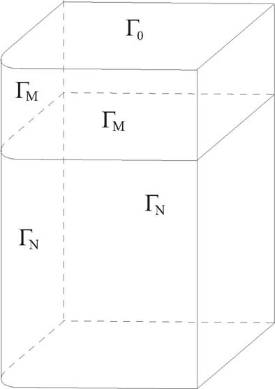
Let Ω¯ ∈ R2 be the rectangular
domain 0,Lx ×0,Ly with round
left-down corner of radius R ≥ 0,
Ω¯= Ω ∪ ∂Ω. Let
V = Ω ×0,Lz be the 3D domain
with boundary Γ = ∂V
which consists of the following parts:
Γ0 = Ω¯ ×0 ,
ΓN = x,y ∈ ∂Ω : x = 0 ∨ y = 0 ×LM,Lz ∪ Ω ×Lz ,
ΓS = x,y ∈ ∂Ω : x≠0 ∧ y≠0 ×0,Lz ,
ΓM = x,y ∈ ∂Ω : x = 0 ∨ y = 0 ×0,LM ,
where 0 ≤ LM < Lz.
In our applied problem domain V
represents a metallic bar (or melt), Ω
is the quarter of z-cross section of a slab,
Lz is the length
of a slab and LM
is the length of primary cooling zone.
We find the temperature field T = T(x,y,z,t)
for (x,y,z) ∈Ω¯
and t ∈ (0,Tf]
( T f is
the time of casting process ending).
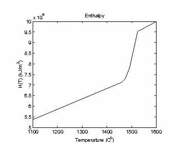
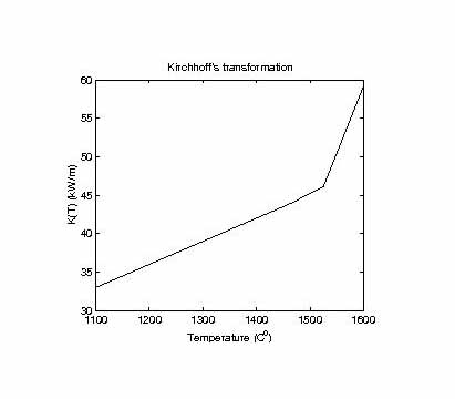
We define the enthalpy function H(T)
and the Kirchoff’s temperature K(T)
by
H T = ρ ∫
0T c ξdξ + L 1 − f
s T,K T = ∫
0T k ξdξ ,
where ρ,
c(T),
k(T) and
L
are density, heat capacity, thermal conductivity and latent heat,
fs T is the solid fraction
at temperature T,
such that
fs T = 1,T > Ts,
0,T < Tl.
Here Ts is the
solidification and Tl
is the melting temperature. On Figures 2, 3 the graphs of enthalpy
function and Kirchhoff’s temperature for steel are presented. Note
that because of the monotonicity and continuity of enthalpy function
H = H(T), we can define the
inverse function T = T(H).
The continuous casting process can be modelled by the following boundary-value
problem:
|
∂H(T)
∂t + v∂H(T)
∂z − ΔK T = 0inV ×0,Tf ,
T = T0onΓ0 ×0,Tf ,
∂K T
∂n + h T − Tw + σɛ T4 − T
ext4 = 0
onΓN ×0,Tf ,
∂K T
∂n = QonΓM ×0,Tf ,
T x,y,z, 0 = T0inV.
| (1) |
Here n is the unit vector
of outward normal to ∂V ,
σ > 0 is the Stefan-Bollzmann
constant, ɛ > 0 is the
emissivity, v > 0 is the
casting speed, h = h x,y,z,t
and Q = Q x,y,z are known
cooling functions, Tw = Tw x,y,z
and Text = Text x,y,z
are known temperatures of cooling liquid and environment,
T f is the
time of casting process ending.
Besides of the temperature-enthalpy formulation (1) we use the following
enthalpy formulation:
|
∂H
∂t + v∂H
∂z − ΔK H = 0inV ×0,Tf ,
H = H(T0)onΓ0 ×0,Tf ,
∂K H
∂n + h T H − Tw + σɛ T4 H − T
ext4 = 0
inΓN ×0,Tf ,
∂K H
∂n = QinΓM ×0,Tf ,
H x,y,z, 0 = H0onV.
| (2) |
Unknown function in (2) is the enthalpy function
H(⋅), by
K(H) we mean
here K(T(H)).
3. Mesh problem and its solving
Let for some ɛ > 0
we know τ = τ ɛ,
such that the following condition holds:
∂H
∂t + v∂H
∂z = H −H˜
τ + ω t, with ∥ω t∥≤ ɛ,∀t : 0 ≤ t < t + τ ≤ Tf,
where H˜ = H x,y,z − vτ,t − τ. In fact, this
means that for this τ the
local ɛ-approximation
of the term ∂H∕∂t + v∂H∕∂z
in a norm ∥⋅∥
is achieved.
The weak formulation of the semi-discrete scheme to problem (1) for a fixed time
level can be written as follows:
|
findH ∈ H1(V ),H ∣
Γ0 = H(T0) :
1
τ ∫
V H T −H˜τηdx + ∫
V ∇K T ⋅∇ηdx+
+ ∫
ΓNh T − Tw + σɛ T4 − T
ext4 ηdx = 0,
∀η ∈ V 0 = v ∈ H1 V : η
Γ0 = 0 .
| (3) |
Here H1 V
is the usual Sobolev space.
Let Ω
be partitioned into a set of quadrilateral finite elements, this triangulation
being topologically equivalent to rectangular one. The triangulation of
Ω and partitioning of
[0, Lz] form the triangulation
of 3D domain V
into a set of prismatic 3D finite elements. Now we can write
the finite element (FEM) discretization of problem (3). Let
V h
be a finite element approximation of the space
H1 (V ), based on the polylinear
elements. Further wh stands
for a V h-approximation
of function w (for a
continuous function w
wh is its
V h -interpolant).
Let
V hT0
= vh ∈ V h V : vh = T0h on Γ0 ,
V h0 = v
h ∈ V h V : vh = 0 on Γ0 .
Approximation of problem (3) by finite element method is defined as
|
1
τ ∫
V Hh Th −H˜hηdx + ∫
V ∇Kh Th ⋅∇ηdx+
+ ∫
ΓNh Th − Tw,h + σɛ T4
h −Text4
h ηdΓN = 0,
∀η ∈ V h0.
| (4) |
Discrete problem (4) is equivalent to the system of nonlinear algebraic equations
(hereafter we use the same notations for continuous and mesh functions):
|
H T −H˜
τ + AK T + B h T − Tw + B T4 − T
ext4 = 0.
| (5) |
Here: A
is the discrete Laplas operator, in current FEM realization
A is the 11-diagonal
matrix; B,B h
are the diagonal matrices with sparse main diagonal.
In enthalpy formulation problem (5) becomes
|
H −H˜
τ + AK H + B h T H − Tw +
+B T H4 − T
ext4 = 0.
| (6) |
Below we consider the problem in enthalpy statement (6). Let
f H = AK H + B h T H − Tw + B T H4 − T
ext4 .
Then an explicit Euler method can be written as
|
Hk+1 = Hk − τk+1f Hk ,H0 = H T0 ,k = 0, 1, 2,…
| (7) |
Here τk are the time steps,
Hk = H t = ∑
i=1kτi is the numerical solution
at the time level t.
The Frechet derivative of the mapping
f H is
given by
J(H) = A ∘ K′(H) + B h ∘ T′(H) + 4B ∘T3(H)T′(H) .
Let λ,ξ is the eigen
pair of operator J,
then
K′ + A−1B hT′ + 4A−1BT3T′ξ = λA−1ξ.
Hereafter we omit the argument H
of functions T,
T ′ and
K′ .
Executing some technical estimates we get the following inequalities:
K′ξ,ξ + A−1B hT′ξ,ξ + 4 A−1BT3T′ξ ≤
≤ LKHλ
maxA A−1ξ,ξ + 4 A−1BT3T′ξ,BT3T′ξ A−1ξ,ξ1∕2+
+ A−1B HT′ξ,B HT′ξ1∕2 A−1ξ,ξ1∕2 ≤
≤ LKHλ
maxA + cond A1∕2L
T H B h +
+4 cond A1∕2L
T HL
T3H A−1ξ,ξ.
Now, maximum eigenvalue of operator
J can
be estimated by
λmax ≤ LKHλ
maxA + cond A1∕2L
T H B h
+4 cond A1∕2L
T HL
T3H.
Here:
- λmaxA
is the maximum eigenvalue of the operator A;
- cond A = λmaxA
λminA
is the condition number of operator A;
- LKH = sup
H∈[H(0),H(Ts)] K′H;
- LT H = sup
H∈[H(0),H(Ts)] T′H;
- LT3H = sup
H∈[H(0),H(Ts)] T3 H.
Let τk = τ
0,
then we have the explicit Euler method with constant step.
Approximation condition in this case is defined by following inequality:
τ0 ≤ τ. Stability condition can
be written as τ0 ≤ cou, where
Courant number cou = 2∕λmax. As it is
known, for large value of λmax
the last condition is too restrictive and too many steps in time can be necessary
when using an explicit scheme.
Let τk
k=1N be a cycle of
time steps in (7), N
be the length of the cycle. The total step of the cycle is
lN (τmax) = ∑
k=1Nτk,
where τmax
is the maximum step of the cycle. The approximation condition of this scheme can
be written as
The relaxed stability condition of this so-called super-time-stepping scheme is
|
∏
k=1N(1 − τ
kλ) < 1∀λ : (λmin ≤ λ ≤ λmax),
| (9) |
where λmin
and λmax
is the minimum and maximum eigenvalues of the operator
J.
To obtain an optimal scheme, a maximum superstep size must be found as maximum
lN (τ(ɛ))
when (8) and (9) hold. An optimal cycle is found by using the
optimal properties of Chebyshev polinomials in [10] for the cases
N = 2p and
N = 2p3q. The
construction of this scheme is based on the using the following parameters:
τmax ≤ τ(ɛ) – the maximum
step of the cycle, cou
– Courant number of the operator.
This scheme is described for the operators with real spectrum. In our problem
operator J
is symmetrizable, thus it has only real spectrum.
In our case we have parameter τf ≫ τ(ɛ)
and we must calculate solution for every time
t = kτf,k = 0, 1, 2,…
It means that we need the time steps cycle such that
lN ≈ τf. Obviously, function
g(x) = ∣τf − lN(x)∣, 0 < x ≤ τ(ɛ) is unimodal for every
fixed N, and it means
that for all fixed ξ > 0
we can easily find τ : g(τ) ≤ ξ.
Values N = 2p
and τ
were defined experimentally. Using explicit scheme with cyclic set of
steps we get some advantage in computing complexity in comparison
with the scheme with a constant step, but it has not a theoretical
N-order advantage, because
we have condition lN ≈ τf.
In the next section we also compare explicit schemes with variable steps
with standard implicit method (see Table 1). The solution of nonlinear
system arising in the implicit scheme was made by Gauss-Seidel method with
preliminary Newton linearization. In column ”Number of iterations” of Table 1 we
present: for the implicit scheme – average number of the iterations required
for the solving of corresponding system of the nonlinear equations at one
time level, for the explicit scheme – number of steps in a cycle. In column
”Time of iteration” the average time of one iteration in milliseconds is
recorded.
4. Optimization problem
The secondary cooling region is divided into
M
cooling zones, in every one the heat transfer coefficient
hk ,k = 1,M¯ have to
be controlled. In optimal control method our aim is to minimize a goal function which
is constructed by means of metallurgical cooling criteria. By these criteria we have two
observation lines on the slab surface (along the corner and center lines of slab surface):
l1 = ((x,y,z) ∈ Γ : x = y = R(1 − 1∕2),z ∈ [LM,Lz]),
l2 = ((x,y,z) ∈ Γ : x = Lx,y = 0,z ∈ [LM,Lz]) and given target
temperatures {tktar,k = 1,M¯¯}
for starting point of each cooling zone along this lines. Let
T tar(x),x ∈ l = l
1 ∪ l2 is the linear
interpolation of {tktar}.
Thus, the goal-function can be defined as
I(T) = 1
2 ∫
l(Ttar − T)2dx.
Let J(T) is the mesh
approximation of I(T),
vector J′(T) is
the derivative of the goal-function. We can formulate the optimal control problem in
the following way:
Find h∗ ∈ U
such that:
|
J(h∗) = min
h∈UJ(h),
| (10) |
where U = {u = (u1,u2,…,uM) : hmin ≤ ui ≤ hmax∀i = 1,M¯}
is the set of constraints for control variables and
T = T(h) is
defined via solution of mesh scheme (6) with the set of variable time steps. Thus, we
have a nonlinear function minimization problem with constraints. To solve problem
(10) we use a gradient method.
To calculate the gradient of the goal-function we construct the adjoint state
problem by using the Lagrange function
L = J(TN)+
+ ∑
k=1N−1Hk+1 − Hk
τk + AK(Tk) + B(h)(Tk − T
w) + B (Tk)4 − T
ext4 ,λk+1.
Here we use the inner product (⋅,⋅)
in the finite dimensional space of vectors. Variation gives
Ly′v = J′(TN) + ∑
k=1N−1vk+1 − vk
τk + A K′(Tk)(Tk)
H′vk ,λk+1+
+ ∑
k=1N−1B(h)(Tk)
H′vk + 4B(Tk)3(Tk)
H′vk,λk+1 = 0.
Obviously,
∑
k=1N−1vk+1 − vk
τk λk+1 = ∑
k=1N−1vk λk
τk −λk+1
τk+1 + vNλN
τN ,λ1 = 0
From here we derive the following system of the linear algebraic equations, which is
the mesh adjoint state problem:
|
λN
τN + J′(TN)(TN)
H′ = 0
λk
τk −λk+1
τk+1 + (Tk)
H′K′(Tk)A∗λk+1 + (Tk)
H′B∗(h)λk+1+
+ 4(Tk)
H′(Tk)3B∗λk+1 = 0,k = N − 1,…, 1.
| (11) |
As it is shown in [10] scheme (11) is stable and stable to round-off errors. Now the
descend direction is defined by
(J′(h))
j = (B(hj)(T − Tw),λ1),
where: hj = 0,…, 0, 1,…, 1︷ ikj
, 0,…, 0T ,j = 1,M¯;
ik j - all mesh points in
the j-th cooling zone.
Vector −J′(h) is the descent
direction. The projection p = (p1,p2,…,pM)
of the vector −J′(h) to
constrains set U
can be calculated as
pi = 0,(hi = hmin ∧ Jj′ > 0) ∨ (h
i = hmax ∧ Jj′ < 0),
−Ji′,otherwize.
Then we consider the one-dimensional minimization problem:
|
ρopt = arg min 0≤ρ≤ρmaxJ(h + ρp),
| (12) |
where maximum descent step ρmax
can be found from: start point h,
current descent direction p
and constraints set U.
In this work we solve (12) by the Brent algorithm of one-dimension minimization
and by the following algorithm:
Step 1.
Let h(ρ) = h + pρ
ρ0 = ρmax
2d ,
where d > 0
is the arbitrary parameter of algorithm
If J(h(ρ0)) > J(h(0))
Then ρopt = 0
End
i = 1
GoTo Step 2
Step 2.
ρopt = ρi−1
ρi = 2ρi−1
If ρi > ρmax
or J(h(ρi)) > J(h(ρi−1))
End
i = i + 1
GoTo Step 2.
The solutions of (10) using both one-dimensional minimization algorithms are the
same, while the second algorithm is much simpler than Brent algorithm.
The results of numerical experiments (optimal control and temperature fields
calculated by using both explicit and implicit schemes) are presented on Figures 4 –
9.
5. Numerical results
Direct solution.
|
|
|
|
| | |
| | |
| | |
| | |
| | |
| | |
| | |
| | |
| | |
| | |
| | |
| | |
| |
| |
| |
| |
| |
| |
| |
| |
| |
| |
| | |
| | |
| |
| |
| |
| | Method | | | Time of one |
| iteration |
| (ms) |
| |
|
|
| Mesh: 11x17x221 |
| Tf = 1000 |
| |
| Explicit scheme | 8 | 116 |
|
| Implicit scheme | 24 | 256 |
|
|
| Explicit scheme | 8 | 56 |
|
| Implicit scheme | 19 | 107 |
|
|
| Explicit scheme | 4 | 28 |
|
| Implicit scheme | 14 | 73 |
|
| |
TABLE 1. Number of iterations and time of calculation for solution of the state
problem.
Optimization.
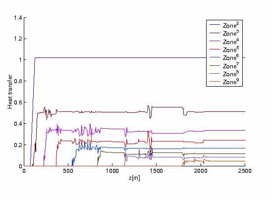 FIGURE 4.
 Optimal cooling control results by implicit scheme
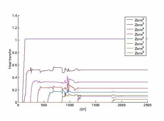 FIGURE 5.
 Optimal cooling control results by explicit scheme
Optimal and target temperatures
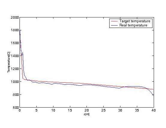 FIGURE 6.
 Temperature by implicit scheme along corner line
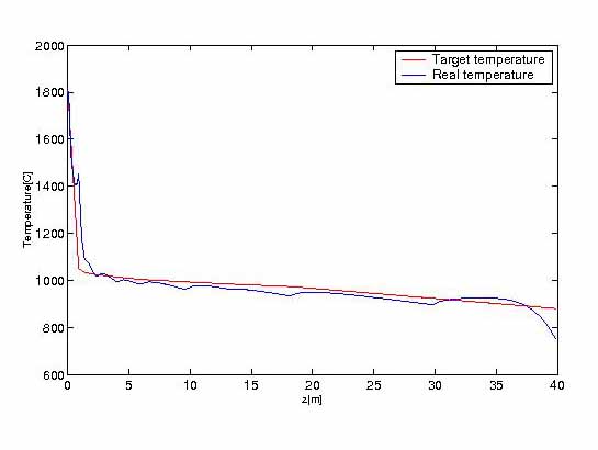 FIGURE 7.
 Temperature by explicit scheme along corner line
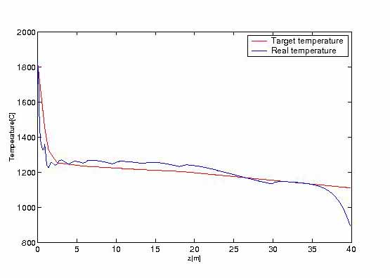 FIGURE 8.
 Temperature by implicit scheme along center line
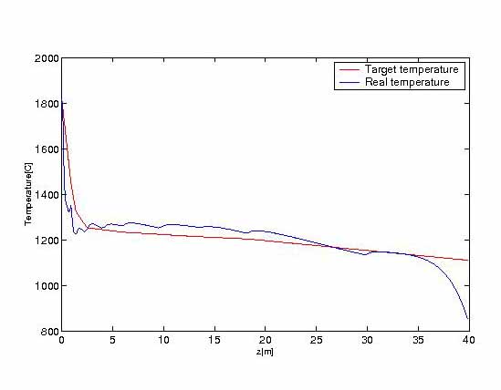 FIGURE 9.
 Temperature by explicit scheme along center line
References
[1] Laitinen E., Neittaanma¨ki
P. On numerical simulation of the continuous casting problem //J. Eng. Math. – 1987.
– V. 22. – P. 335–354.
[2] Louhenkilpi S., Laitinen E., Nieminen R. Real time simulation of heat transfer in
continuous casting // Metall. Trans. B. – 1993. – V. 24B. – P. 685–693.
[3] Rodrigues J. F., Yi F. On a two-phase continuous casting Stefan problem with nonlinear
flux // Euro J. App. Math. – 1990. – V. 1. – P. 259–278.
[4] Chen Z., Jiang L. Approximation of a two phase continuous casting problem // J. Part.
Diff. Equations. – 1998. – V. 11. – P. 59–72.
[5] Laitinen E., Lapin A. Implicit approximation and iterative solution for the continuous
casting problem // Preprint, July, 1999, Dep. of Math. Sci., University of Oulu. – 1999.
– 17 p.
[6] Laitinen E., Lapin A., Pieska¨
J. Mesh approximation and iterative solution of the
continuous casting problem // in: ENUMATH 99. Ed. by P.
Neittaanma¨ki,
T. Tiihonean and P. Tarvainen. World Scientific, Singapore. – 2000. – P. 601–617.
[7] Laitinen E., Saranen J., Pieska¨
J., Lapin A. Comparison of domain decomposition methods for solving continuous
casting problem // in: Domain Decomposition Methods DDM-13. Ed. by N. Debit, M.
Garbey, R. Hoppe, J. Periaux, D. Keyes, Y. Kuznetsov. CIMNE, Barselona. – 2002. –
P. 411–418.
[8] Laitinen E., Lapin A., Pieska¨
J. Asinchronous domain decomposition methods for solving continuous casting problem
// J. of Comp. and Appl. Math. – 2003. – V. 154. – P. 393–413.
[9] Dautov R.Z., Ignatieva M.A. Multigrid solution of a two-phase Stefan problem with
prescribed convection // Proceedings of Russian-Finnish Workshop: Numerical methods
for continuous casting and related problems, V. 9. – Kazan, DAS Publisher, 2001, –
pp. 3-11.
[10] Lebedev V.I. Functional analysis and calculus mathematics. – M.: Science, 2000. – 290
P.
[11] Lebedev V.I. Explicit difference schemes for solving stiff systems of ODEs and PDEs
with complex spectrum//Russ. J. Numer. Anal. Math. Modelling. – 1998. – V. 13. – No 2.
– P. 107–116.
[12] Lebedev V.I. Explicid difference schemes for solving stiff schemes with complex or
partitioned spectrum//JNM and MP. – 2000. – V. 40. – No 12. – P. 1801–1812.
KAZAN STATE UNIVERSITY, RUSSIA
UNIVERSITY OF OULU,FINLAND
KAZAN STATE UNIVERSITY, RUSSIA
E-mail address: alapin@ksu.ru
Received October 15, 2003