Lobachevskii Journal of Mathematics Vol. 13, 2003, 67 – 80

©E. Laitinen, A.V. Lapin, and J. Pieska¨

E. Laitinen, A.V. Lapin, and J. Pieska¨
NUMERICAL EXPERIMENTS WITH MULTILEVEL SUBDOMAIN DECOMPOSITION METHOD

________________

Key words and phrases. Stefan problem, continuous casting process, finite element method, predictor-corrector scheme, domain decomposition.

This work is supported by RFBR, project N 01-01-00068.

ABSTRACT. In this paper, we present a new numerical approach to solve the continuous casting problem. The main tool is to use so-called IPEC method and DDM similar to [6] with multilevel domain decomposition. On the subdomains we use the multidecomposition of the subdomains. The IPEC is used both in the whole calculation domain and inside the subdomains. Calculation algorithm is presented and numerically tested. Several conclusions are made and discussed.

1. Introduction

Theory of the so-called regional-additive schemes (splitting schemes with domain decomposition) for linear diffusion and convection-diffusion have been studied in [14],[15] and [16]. The stability have been proved and error estimates have been deduced. For the non-linear problems like our their technique is not available.

Several new finite-difference schemes for a nonlinear convection-diffusion problem are constructed and numerically studied in [6]. These schemes are constructed on the basis of non-overlapping domain decomposition and predictor-corrector approach. (Note that the term “predictor-corrector domain decomposition method” was introduced by Quarteroni and Valli [13]).

The paper of Lapin and Pieska¨ [6] was motivated by [2], [9], [10], [11], where TL¹ , EP² and EPIC³ methods have been studied and tested. The EPIC method was proved to be stable and scalable when solving on a big number of processors. In the paper [6] the scheme from [10], [11] was modified in such a way, that its implementation leads to IPEC⁴ method.

The main idea of these kind of algorithms is first to solve the problem in artificial boundaries predictor step). After the solution at the boundaries is known then it can be used as a Dirichlet-type boundary condition and the non-coupled subdomain problems can be solved in parallel. The last step of these methods is to correct the solution at the artificial boundaries (corrector step). The idea is similar to Schur’s complement type methods but in our approach the calculation of the artificial boundaries between subdomains are very easy and cheap to perform. There is also no need to construct a good preconditioner for the interface problems.

The advantages of predictor-corrector methods (IPEC or EPIC) is that we reduce the amount of information sending between processors. We need to send only once the subsolutions from slave processors to master processor. When we use Schwarz alternating methods with the overlapping subdomains, the number of sending and receiving is much more bigger. The numerical experiences show that the speedup of IPEC method is very good comparing with Schwarz methods and calculation times are roughly half of the times of Schwarz methods. Moreover, the linear speedup is reached in the numerical tests of [6].

The idea of multidecomposition method MDD is to use DDM with IPEC inside the subdomains. The subdomain is divided into smaller subdomains and then IPEC method is used to solve these smaller subproblems sequently.

The rest of the article is organized as follows. In the section 2 we present the continuous casting problem. The section 3 deals with the mesh approximation of the problem. The used domain decomposition and calculation algorithm is presented in the section 4. The section 5 is devoted to numerical testing of the new algorithm. Finally, in the section 6 the conclusions are made.

2. Problem statement

The continuous casting problem can be mathematically formulated as follows. Let the rectangular domain Ω ⊂ ℝ2, Ω = (0,l 1) × (0,l2) be occupied by a thermodynamically homogeneous and isotropic steel. We denote by H ̄ (x,t) the enthalpy related to the unit mass and by T(x,t) the temperature for (x,t) ∈Ω ̄ × [0,tf]. We have constitutive law

H ̄ = H ̄ (T) = ρ \int 0 T c (Θ) d Θ + ρ L (1 - f s (T)),

where ρ is the density, c(T) is the specific heat, L is the latent heat and fs (T) is the solid fraction at temperature T of the form

fs(T) = 1 for T < TS, TL − T TL − TS, for TS < T < TL, 0 for T > TL.

The graph H̄(T) is an increasing function ℝ → ℝ, involving near vertical segment, which corresponds to a phase transition state, namely, for T ∈ [TS,TL]. In the case of piecewise constant specific heat c(T), the enthalpy function is piecewise linear of the form

H̄(T) = ᾱ1T + β̄1 for T < TS, ᾱ2T + β̄2, for TS < T < TL, ᾱ3T + β̄3 for T > TL.

Further by k(T) we denote the thermal conductivity coefficient, which is continuous and increasing in T.

A continuous casting process can be described by a boundary-value problem, formally written in the following pointwise form: find T (x,t) and H ̄ (x,t) such that

\partial H ̄ \partial t + v \partial H ̄ \partial x 2 - \nabla \cdot (k (T) \nabla T) = 0 for x \in Ω, t > 0, T = z ̄ (x, t) for x \in Γ D, t > 0, k (T) \partial T \partial n = g, for x \in Γ N, t > 0, H ̄ = H ̄ 0 (x) for x \in Ω ̄, t = 0,

where v = const > 0 is a casting speed in x2-direction, ΓD ∪ ΓN = ∂Ω is the boundary of the domain, below ΓD = {x ∈ ∂Ω : x2 = 0 ∨ x2 = l2}.

Using Kirchoff’s transformation u = K(T) = ∫ 0T k(ξ)dξ and the notation H(u) = H̄(T) = H̄(K−1(u)), we can rewrite the continuous casting problem as

(P) \partial H \partial t + v \partial H \partial x 2 - Δ u = 0, for x \in Ω, t > 0, u = z (x, t) for x \in Γ D, t > 0, \partial u \partial n = g, for x \in Γ N, t > 0, H = H 0 (x) for x \in Ω ̄, t = 0,

The existence and uniqueness of a weak solution for problem (P) are proved in [12].

In the case of piecewise constant specific heat c(u) the enthalpy function takes the form

H(u) = α1u + β1 for u < uS, α2u + β2, for uS < u < uL, α3u + β3 for u > uL.

(1)

3. Mesh approximation of continuous casting problem

We approximate problem (P) by an implicit in time finite difference scheme and by a semi-implicit finite difference scheme, using for the approximation in space variables a finite element method with the quadrature rules.

Let Ξh be a partitioning of Ω in the rectangular elements δ of dimensions h1 × h2 and V h = {uh(x) ∈ H1(Ω) : u h(x) ∈ Q1 for all δ ∈ Ξh}, where Q1 is the space of bilinear functions. By Πhv(x) we denote the V h-interpolant of a continuous function v(x), i.e. Πhv(x) ∈ V h and coincides with v(x) in the mesh nodes (vertices of all δ ∈ Ξh). We also use an interpolation operator Ph, which is defined as follows: for any continuous function v(x) the function P h v(x) is piecewise linear in x1, piecewise constant in x2 and on δ = [x1,x1 + h1] × [x2,x2 + h2] it coincides with v(x) at (x1,x2 + h2) and (x1 + h1,x2 + h2).

Let further V h0 = {u h(x) ∈ V h : uh(x) = 0 for all x ∈ ΓD}, V h z = {u h(x) ∈ V h : uh(x) = zh for all x ∈ ΓD}. Here zh is the bilinear interpolation of z on the boundary ΓD. For any continuous function v(x) we define the quadrature formulas:

S δ (v) = \int δ Π h v d x, S \partial δ (v) = \int \partial δ Π h v d x, E δ (v) = \int δ P h v d x,

S Ω (v) = \sum δ \in Ξ h S δ v, S Γ 2 (v) = \sum \partial δ \in Ξ h \cap Γ ̄ 2 S \partial δ (v), E Ω (v) = \sum δ \in Ξ h E δ (v) .

Let also ωτ = {tk = kτ, 0 ≤ k ≤ M,Mτ = tf} be an uniform mesh in time on the segment [0,tf] and ∂t ̄H = 1 τ(H(x,t) − H(x,t − τ)). Then the implicit in time finite difference scheme with up-wind approximation of the convective term v∂H∕∂x2 can be written as follows: for all t ∈ ωτ, t > 0, find uh ∈ V hz and Hh ∈ V h such, that

SΩ(∂t ̄Hhηh) + EΩ(v∂Hh ∂x2 ηh) + SΩ(∇uh∇ηh) = SΓ2(gηh) for all ηh ∈ V h0.

(2)

When constructing the characteristic mesh scheme we approximate the term ∂ ∂t + v ∂ ∂x2H by using the characteristics of the first order differential operator (similar to [1], [3]). Namely, if (x1 ,x2,t) is the mesh point on the time level t we choose x˜2 = x2 −∫ t−τtv(ξ)dξ and approximate:

\partial \partial t + v \partial \partial x 2 H \approx 1 τ H (x 1, x 2, t) - H ˜ (x 1, x 2, t - τ),

where we denote H˜(x,t − τ) = H(x1,x˜2,t − τ).

Near the boundary it can happen that x ˜ 2 < 0. In that case we put H˜(x,t − τ) = H(x1, 0,t − τ). In what follows we use the notation dt ˜H = 1 τ(H(x,t) −H˜(x,t − τ)) for the difference quotient in each mesh point on time level t.

Now, the characteristic finite difference scheme for problem (P) is: for all t ∈ ωτ, t > 0, find uh ∈ V hz and Hh ∈ V h such that

SΩ(dt ˜Hhηh) + SΩ(∇uh∇ηh) = SΓ2(gηh) for all ηh ∈ V h0

(3)

Let N0 = card V h0 and u ∈ ℝN0 be the vector of nodal values for uh ∈ V h0. We use the writing uh ⇔ u for this bijection. We define N0 × N0 matrices by the following relations: for all u,η ∈ ℝN0,u ⇔ u h ∈ V h0 and η ⇔ η h ∈ V h0,

(Ã u, η) = S Ω (\nabla u h \nabla η h), (M u, η) = S Ω (u h η h), (C ˜ u, η) = E Ω (v \partial u h \partial x 2 η h),

A 0 = M - 1 Ã, C = M - 1 C ˜ .

Let now z˜h(x) ∈ V h be the function, which is equal to zh on Γ ̄D and 0 for all nodes in Ω ∪ ΓN. Then a vector f is defined by the equality

(f,η) = SΓ2(gηh) − SΩ(∇z˜h,∇ηh)∀η ∈ ℝN0 ,η ⇔ ηh ∈ V h0,

and we set F = M−1f.

In these notations the algebraic form for implicit mesh scheme (2) at fixed time level is:

∂t ̄H + A0u + CH = F,

(4)

while characteristic mesh scheme (3) becomes

dt ˜H + A0u = F,

(5)

It is easy to see, that A0 is the standard five-point finite difference approximation of Laplace operator, A0 u = −ux1x̄1 − ux2x̄2 for the internal mesh points with the notations ux1 = h−1(u(x 1 + h1,x2) − u(x1,x2)),ux̄1 = h−1(u(x 1,x2) − u(x1 − h1,x2)), and similarly for ux2 and ux̄2. For more detailed writing of the explicit form for A0 u let us introduce several sets of the grid points. Namely, let ω ̄ be the set of all grid points, i.e. vertices of finite elements, γD = Γ ̄D∩ω̄,γN = ΓN∩ω̄,ω = Ω∩ω̄,γN− = {x ∈ γ N : x1 = 0},γN+ = {x ∈ γ N : x1 = l1}.

Now A0 = A1 + A2 with

A 1 u = - u x 1 x ̄ 1 for x \in ω, - 2 h 1 - 1 u x 1 for x \in γ N -, 2 h 1 - 1 u x ̄ 1 for x \in γ N +,

A 2 u = - u x 2 x ̄ 2 for x \in ω \cup γ N, 0 for x \in γ D .

The term CH in the implicit scheme corresponds to an up-wind approximation of the nonlinear convective term, CH = Hx̄2 for x ∈ ω ∪ γN.

4. Domain decomposition by straight lines

In this section we present the IPEC algorithm [6]. We restrict our discussion to the case of decomposition by unidirect straight lines. More variations and possibilities of decomposition are discussed and tested in [6]. Methods presented here and in the following section can be easily implemented and used with more complicated decompositions of calculation domain. Moreover, the generalization to 3-D case is straightforward. In that case the 1-D lines are replaced by 2-D planes.

Let the domain Ω be decomposed into two subdomains Ω1 and Ω2 by a straight line Sy in x2 -direction, which is also a grid line. We denote by δSy the characteristic function of this line, i.e., the mesh function δSy (x) = 1 for x ∈ Sy ∩ω̄, while δSy (x) = 0 for other mesh points. Also, let ω̄k,k = 1, 2 be the corresponding to the subdomains Ω ̄k sets of grid points, Sy being the common part of their boundaries.

Let A2u = −δSyux1x̄1 and A1 = A0 − A2,

A 1 u = - (1 - δ S y) u x 1 x ̄ 1 - u x 2 x ̄ 2 for x \in ω, - 2 h 1 - 1 u x 1 - u x 2 x ̄ 2 for x \in γ N -, 2 h 1 - 1 u x ̄ 1 - u x 2 x ̄ 2 for x \in γ N + .

Now, instead of implicit scheme (4) we consider the following scheme on the time level tn+1 = (n + 1)τ:

1 τ(Hn+1∕2 − Hn) + A 1un+1∕2 + A 2un + CHn+1∕2 = F,

(6)

δSy τ (Hn+1 − Hn) + 1 − δSy τ (Hn+1 − Hn+1∕2)+ δSyA1un+1∕2 + A 2un+1 + δ SyCHn+1 = δ SyF.

(7)

Similarly, characteristic scheme (5) is changed by

1 τ(Hn+1∕2 −H˜n) + A 1un+1∕2 + A 2un = F,

(8)

δSy τ (Hn+1 −H˜n) + 1 − δSy τ (Hn+1 − Hn+1∕2) + δ SyA1un+1∕2 + A 2un+1 = δ SyF.

(9)

Let us discuss the implementation of scheme (6),(7). In the points of Sy first equation of (6) has the form:

Hn+1∕2 − Hn τ − ux2x̄2n+1∕2 − u x1x̄1n + H x̄2n+1∕2 = F,

(10)

i.e. in the points of Sy we have one-dimensional problem (10), that we solve first. After, the rest part of the first equation in (6) is splitted into two non-coupled implicit schemes in the subdomains:

Hn+1∕2 − Hn τ − ux1x̄1n+1∕2 − u x2x̄2n+1∕2 + H x̄2n+1∕2 = F, for x ∈ ω 1 ∪ ω2, Hn+1∕2 − Hn τ − 2 h1ux1n+1∕2 − u x2x̄2n+1∕2 + H x̄2n+1∕2 = F, for x ∈ γ N−, Hn+1∕2 − Hn τ + 2 h1ux̄1n+1∕2 − u x2x̄2n+1∕2 + H x̄2n+1∕2 = F, for x ∈ γ N+

(11)

and these equations are accomplished by Dirichlet boundary conditions, given on γD and calculated from (10) on Sy.

Further, it is easy to check, that for the points x∉Sy the second equation (7) coincide with (11) and has the same Dirichlet boundary conditions on γD and on Sy, so, un+1(x) = un+1∕2(x) for x∉Sy and it makes no sense to solve these equations. It remains only to solve the system of the equations, corresponding to x ∈ Sy:

Hn+1 − Hn τ − ux2x̄2n+1∕2 − u x1x̄1n+1 + H x̄2n+1∕2 = F.

As un+1(x) = un+1∕2(x) for x∉Sy, this system becomes

Hn+1 − Hn τ + Hx̄2n+1∕2 + 2un+1(x 1,x2) h12 − ux2x̄2n+1∕2 −un+1∕2(x 1 − h1,x2) + un+1∕2(x 1 + h1,x2) h12 = F,x ∈ Sy,

(12)

i.e. we get the system of scalar equations for (un+1(x),Hn+1(x)),x ∈ S y.

Thus, the algorithm for the implementation of (6),(7) consists of 3 steps:

1):: Predictor step: solving one-dimensional problem (10);
2):: Main step: concurrent solving subproblems (11);
3):: Corrector step: solving the system of scalar equations (12).

With the slight modifications the implementation of scheme (8),(9) is similar. Namely, in the points of Sy first equation of (8) has the form:

Hn+1∕2 −H˜n τ − ux2x̄2n+1∕2 − u x1x̄1n = F,

(13)

i.e. in the points of Sy we have one-dimensional problem (13), that we solve first. After that the rest part of first equation in (8) is splitted into two non-coupled characteristic schemes in the subdomains:

Hn+1∕2 −H˜n τ − ux1x̄1n+1∕2 − u x2x̄2n+1∕2 = F, for x ∈ ω 1 ∪ ω2, Hn+1∕2 −H˜n τ − 2 h1ux1n+1∕2 − u x2x̄2n+1∕2 = F, for x ∈ γ N−, Hn+1∕2 −H˜n τ + 2 h1ux̄1n+1∕2 − u x2x̄2n+1∕2 = F, for x ∈ γ N+

(14)

and these equations are accomplished by Dirichlet boundary conditions, given on γD and calculated from (13) on Sy.

Finally it remains to solve the system of the equations, corresponding to x ∈ Sy:

Hn+1 −H˜n τ − ux2x̄2n+1∕2 − u x1x̄1n+1 = F.

As un+1(x) = un+1∕2(x) for x∉Sy, this system becomes

Hn+1 −H˜n τ + 2un+1(x 1,x2) h12 − ux2x̄2n+1∕2 −un+1∕2(x 1 − h1,x2) + un+1∕2(x 1 + h1,x2) h12 = F,x ∈ Sy,

(15)

i.e. we get the system of scalar equations for (un+1(x),Hn+1(x)),x ∈ S y.

Remark 1. Above we assumed that the calculation domain Ω is divided into two parts Ω1 and Ω2. This is not restrictive and we refer to [6] for more detailed discussion of the decomposition into several subdomains, also with corner and cross points. Even the case of curvilinear decomposition is studied in [6] and found to be stable and accurate under the natural assumptions for the mesh parameters.

Remark 2. We consider the 2D-case. The proposed methods have natural extensions to the 3D-case. We notice that in predictor and corrector steps the one-dimensional problems corresponding to the mesh line Sy are replaced by the two-dimensional problems corresponding to a plane Sxy.

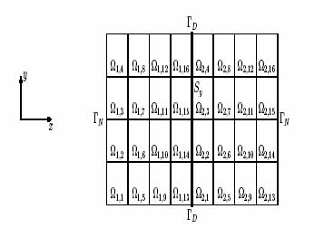
4.1. Multidecomposition method. The general idea of the multidecomposition is to divide the subdomain to smaller subdomains i.e. we use two-level decomposition of the calculation domain. The main reason is to decrease the algebraic size of the problems and thus make the calculation times much smaller. The division of the subdomains is presented in the figure 1. The idea of using multilevel decomposition is not new but the technique presented in this paper gives a good and effective method when solving large complex time dependent problems.

Figure 1:

Used nonoverlapping domain decomposition and multidecomposition of the subdomains.

We use the notation Ωi = ⋃ ji=1pi Ωi,ji. The calculation algorithm for characteristic mesh scheme (13)-(15) is presented below. The algorithm for implicit mesh scheme (10)-(12) is similar.

Algorithm 1.

:
1.:: On a time level n perform on the main processor the predictor step (13) on the artificial boundary Sy.
2.:: Send the values of un+1∕2 and Hn+1∕2 on the boundary Sy to the slave processors.
3.:: Concurrently on the slave processors perform the predictor step (13) on the artificial boundaries of the subdomains Ωi,ji,i = 1, 2,j1 = 1,...,p1,j2 = 1,...,p2.
4.:: Concurrently on the slave processors perform sequentially the main step (14) on the subdomains Ωi,ji.
5.:: Concurrently on the slave processors perform the corrector step (15) on the artificial boundaries of the subdomains Ωi,ji,i = 1, 2,j1 = 1,...,p1,j2 = 1,...,p2.
6.:: Send the values of un+1 and Hn+1 from slave processors to the master processor.
7.:: On the main processor perform the corrector step (15) on the artificial boundary Sy.
8.:: Put n = n + 1, if the final time tf is reached then STOP, else GOTO 1.

Remark 3. On the step 3. of the algorithm 1 we do not do the predictor step (13) on the artificial boundary Sy.

Remark 4. On the steps 3.-5. we do the calculations concurrently. However, we do not synchronize our calculation in such a way that all processors move from step to another at the same time. The step 6. is synchronization point and it is performed at the same time.

The use of high number of subdomains inside the subdomain may increase the error dramatically. To overcome this feature we introduce so called smoothing steps to our method. Namely, our algorithm 1 is replaced by the following one.

Algorithm 2.

:
1.:: On the time step n perform on the main processor the predictor step (13) on the artificial boundary Sy.
2.:: Send the values of un+1∕2 and Hn+1∕2 on the boundary Sy to the slave processors.
3.:: Concurrently on the slave processors perform the predictor step (13) on the artificial boundaries of the subdomains Ωi,ji,i = 1, 2,j1 = 1,...,p1,j2 = 1,...,p2.
4.:: Concurrently on the slave processors perform sequentially the main step (14) on the subdomains Ωi,ji.
5.:: Concurrently on the slave processors perform the corrector step (15) on the artificial boundaries of the subdomains Ωi,ji,i = 1, 2,j1 = 1,...,p1,j2 = 1,...,p2.
6.:: On the slave processors perform the smoothing step i.e. few iterations of the MSOR-method (modified SOR-method) over the whole subdomain Ωi.
7.:: Send the subsolutions un+1 and Hn+1 from slave processors to the main processor.
8.:: On the main processor perform the corrector step (15) on the artificial boundary Sy.
9.:: On the master processor perform few iterations of the MSOR-method in the neighborhood of Sy.
10.:: Put n = n + 1, if the final time tf is reached then STOP, else GOTO 1.

Remark 5. In the algorithm 2 we use the smoothing on steps 6. and 9. According to our knowledge the good amount of MSOR-iterations is less than 10. This amount ensures the reducing of the error and do only slightly increase the calculation time.

Remark 6. The step 9. in the algorithm 2 is performed in the neighborhood of the artificial boundary Sy. The good width of the smoothing area is about 10 grid lines i.e from artificial boundary 5 grid lines to both directions.

Remark 7. In both algorithms 1 and 2 we use the predictor step 3. and corrector step 5. which require the decomposition along and against the convection. There are also cross points. In the article of Lapin and Pieska¨ [6] are discussed more carefully the implementation of such kind of decomposition.

Remark 8. The use of only two subdomains and processors is not restrictive. The usage of more processors and subdomains is straightforward. The numerical results presented in the section 5 verify this.

4.2. Multidecomposition method with one processor. The multidecomposition algorithms 1 and 2 are very effective and extremely quick in the case of many processors. We used the idea of multidecomposition for the situation where we have only one processor. Now we do not have artificial boundaries which decouples problem into subproblems. Anyway, we still have boundaries between subdomains inside the whole domain. The multidecomposition algorithm for one processor with characteristic mesh scheme read as follows.

Algorithm 3.

:
1.:: On every time level n perform the predictor step (13) on the artificial boundaries of the subdomains Ω1,j,j = 1,...,p.
2.:: Perform sequentially the main step (14) on the subdomains Ω1,j.
3.:: Perform the corrector step (15) on the artificial boundaries of the subdomains Ω1,j,j = 1,...,p.
4.:: Perform the smoothing step i.e. few iterations of the MSOR-method over the whole calculation domain Ω.
5.:: Put n = n + 1, if the final time tf is reached then STOP, else GOTO 1.

5. Numerical experiments with one processor

Let Ω =]0, 1[×]0, 1[ with the boundary Γ divided in two parts such that ΓD = {x ∈ ∂Ω : x2 = 0 ∨ x2 = 1} and ΓN = Γ ∖ ΓD, moreover let tf = 1. Let us consider the case where the phase change temperature uSL = 1 and the latent heat L = 1. Let the phase change interval be [uSL − ɛ,uSL + ɛ], ɛ = 0.01, and the velocity is v(t) = 1 5. Our numerical example is

∂H ∂t − ΔK + v(t)∂H ∂x2=f(x; t) on Ω, u(x1,x2; t)=(x1 −1 2)2 −1 2e−4t + 5 4 on ΓD, ∂u ∂n=1 on ΓN, u(x1,x2; 0)=(x1 −1 2)2 + (x 2 −1 2)2 + 1 2 on Ω,

where Kirchoff’s temperature is according to it’s definition

K(u) = u if u < uSL − ɛ, 3 2u −1−ɛ 2 if u ∈ [uSL − ɛ,uSL + ɛ], 2u − 1 if u > uSL + ɛ,

and enthalpy

H(u) = 2u if u < uSL − ɛ, 1+8ɛ 2ɛ (u − 1) + 5+4ɛ 2 if u ∈ [uSL − ɛ,uSL + ɛ], 6u − 3 if u > uSL + ɛ.

Furthermore, let the known right-hand side be

f(x; t) = 4e−4t + 1 5(4x2 − 2) − 4 if u < uSL, 12e−4t + 1 5(12x2 − 6) − 8 if u > uSL.

The exact solution of our problem is

u(x1,x2; t) = (x1 −1 2)2 + (x 2 −1 2)2 −1 2e−4t + 1.

The stopping criterion of the calculations was the L2 -norm of residual: ∥r∥L2(Ω) < 10−4. We divide the domain Ω into non-overlapping subdomains Ωi presented in the figure 1.

We tested algorithm 3 in two different cases. First, we fixed the number of grid points and changed the number of inner subdomains. The calculation grid was 129 × 129 in space and we took 256 time steps. The calculation times for different number of inner subdomains are presented in the table 1.


♯ of inside subdomains	Time [s]

1 × 1	112.9 s
2 × 2	76.2 s
3 × 3	66.1 s
4 × 4	56.9 s
8 × 8	39.9 s

Table 1:

Calculation times in seconds for MDD when the grid size is fixed and number of inside subdomains are changed.

In the table 1 the 1 × 1 subdomain division means the calculation times for MSOR method for the whole calculation domain.

In the second test case we changed the calculation grid and number of time steps. We fixed the number of inner subdomains to be 4 × 4. For many calculation grid this decomposition is not the optimal one but it very clearly emphasizes the advantage of MDD. The results are in the table 2.


Grid	SEQ	MDD

65 × 65 × 128	8.67 s	4.75 s
129 × 129 × 256	112.9 s	56.9 s
257 × 257 × 512	1425 s	687 s

Table 2:

Calculation times in seconds for sequential MSOR (SEQ) and MDD when the calculation grid is changed.

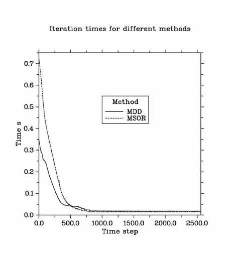
In the figure 2 we measured the time which different algorithms (MSOR and MDD) spend at different time levels. In this case we had the grid size 129 × 129. Normally for this kind of mesh we would take 256 times steps. Now we liked to test how these methods behave when the solution goes to steady-state situation. We took 2560 time steps i.e. 10 times more than usually to see the behavior. The MDD is much better comparing to MSOR in the beginning of the calculations when we have big changes in our simulation.

When time increases the calculation time drop very rapidly and both methods spend equal amount of time for each time step. This is good result for MDD because it is very effective for the case when we have big changes. Near steady-state situation it is as good as MSOR.

Figure 2:

Time spend on each time level for different methods.

6. Conclusions

The numerical examples show that the multidecomposition method (MDD) is very effective numerical method when solving continuous casting problem. The idea to divide the subdomains to smaller subdomains seems to be very good and profitable. The algebraic dimensions of the subproblems inside the subdomains are very small and thus they are very quick to solve. The dimension is in many cases so small that even direct solvers could be effective.

The numerical results for one processor seem to be very promising. We do not need to have big parallel computers to achieve advantages of parallel computer. Only few processors are enough and in some cases even only one processor is good. The table 2 very clearly shows the advantages of MDD. In that table the decomposition is clearly not optimal. The table 1 is good indicator to that. Anyhow, even with poor knowledge of the problem MDD method can be used. When the system is stable and big changes do not appear (like the number of grid points changes or time step changes) then MDD can be optimized good and numerical advantages comparing with MSOR method in the case of one processor and with additive Schwarz alternating method in the case of many processor becomes very dramatical.

References

[1] Z. Chen, Numerical solutions of a two-phase continuous casting problem, Numerical Methods for Free Boundary Problem, P. Neittaanma¨ki, eds. International Series of Numerical Mathematics 99., Birkha¨user, Basel., pp. 103-121, 1991.

[2] C. N. Dawson, Q. Du and T. F. Dupont, A finite difference domain decomposition algorithm for numerical solution of the heat equation, Mathematics of Computation, vol. 57, pp. 63-71, 1991.

[3] J. Jr. Douglas and T.F. Russel, Numerical methods for convection-dominated diffusion problem based on combining the method of characteristic with finite element or finite difference procedures, SIAM J. Numer. Anal., V. 19., pp. 871-885, 1982.

[4] E. Laitinen and A.V. Lapin, Semi-Implicit Mesh Scheme and Splitting Iterative Methods for the Solution of Continuous Casting Problem, Preprint, University of Oulu, Finland, 19p., 1999

[5] E. Laitinen, A.V Lapin and J. Pieska¨, Splitting iterative methods and parallel solution of variational inequalities, Lobachevskii Journal of Mathematics, Vol. 8, p. 167-184, 2001. http://ljm.ksu.ru/vol8/latin.htm

[6] A.V Lapin and J. Pieska¨, On the parallel domain decomposition algorithms for time-dependent problems, Lobachevskii Journal of Mathematics, Vol. 10, p. 27-44, 2002. http://ljm.ksu.ru/vol10/lpp.htm

[7] A.V. Lapin and D.O. Solovyev, Splitting iterative methods for variational inequalities, Preprint No 783, Center of Calcul., Novosibirsk, 24 p., 1988

[8] J.M Ortega and W.C. Rheinboldt, Iterative solution of nonlinear equations in several variables, Academic Press Inc. Orlando, Florida 1970.

[9] W. Rivera, J. Zhu and D. Huddleston, An efficient parallel algorithm with application to computational fluid dynamics, To be appear in Computers and Mathematics with Applications.

[10] W. Rivera and J. Zhu, A scalable parallel domain decomposition algorithm for solving time dependent partial differential equations, Proceedings of the International Conference on Parallel and Distributed Processing Technology and Applications, edited by H. R. Arabnia, CSREA Press, Athens GA, pp. 240-246, 1999.

[11] W. Rivera, J. Zhu and D. Huddleston, An efficient parallel algorithm for solving unsteady nonlinear equations, Proceedings of the International Conference on Parallel Processing Workshops, edited by T. M. Pinkston, IEEE Computer Society, Los Alamitos, California, pp. 79-84, 2001.

[12] J. F. Rodrigues and F. Yi, On a two-phase continuous casting Stefan problem with nonlinear flux, Euro J. App. Math., V. 1., pp. 259-278, 1990.

[13] A. Quarteroni and A. Valli, Domain decomposition methods for partial differential equations, Clarendon Press Oxford, New York 1999.

[14] A.Samarskii, P.Vabischevich, Finite difference schemes with operator multipliers, Minsk, Institute of Mathematics of Belorussia, 442pp, 1998.

[15] A.Samarskii, P.Vabischevich, Factorized regional-additive schemes for convection-diffusion problems (in Russian), Reports of Rusian Acad.Sciences (Mathematics), 1996, V.346, P/742-745.

[16] P.Vabischevich, Parallel domain decomposition algorithms for time-dependent problems of mathematical physics , Advances in Numerical Methods and applications. Singapore: World scientific, 1994, P.293-299.

UNIVERSITY OF OULU, FINLAND.

KAZAN STATE UNIVERSITY, RUSSIA.

E-mail address: alapin@ksu.ru

UNIVERSITY OF OULU, FINLAND.

ReceivedOctober 15, 2003