First order systems

2.2 First order systems

We shall now restrict consideration to systems which have at most one space derivative, i.e. systems of the form,

Using the above theorem, it is easy to see that if a system $P (D )$ is well posed, then so is the system $P (D ) + B$ , where $B$ is any constant matrix. For the particular case at hand, this means that we can further restrict attention, without loss of generality, to the the principal part of the operator, namely

P1 (D ) := AaDau,

where $a A$ is a $s × s$ matrix valued vector in $n ℜ$ . In this case we can improve on the above condition by showing that well posedness implies no growth of the solution, that is that we can choose $α = 0$ above.

Theorem 3 A first order system is well posed if and only if there exist, a constant $k$ , and a positive definite Hermitian form $H (ω )$ such that:

k− 1I ≤ H (ω) ≤ kI and H (ω)Aa ωa − Aa⋆ωaH (ω) = 0 ∀ωa with |ωa | = 1.

If $Aa$ satisfies the above condition for some $H (ω )$ , then we say that $P (D )$ is strongly hyperbolic, which, as we see, is equivalent for first order equation systems to well posedness. If the operator $H$ does not depend on $ωa$ , a case that appears in most physical problems, then we say the system is symmetric hyperbolic. Indeed, if $H$ does not depend on $ωa$ , then there is a base in which it just becomes the identity matrix. (One can diagonalize it and re-scale the base.) Then the above condition in the new base just means that $Aa ωa$ – with the upper matrix index lowered – is symmetric for any $ωa$ , and so each component of $Aa$ is symmetric. Even in the general (strongly hyperbolic) case, one can find a base ( $ωa$ dependent) in which $P (iω )$ can be diagonalized, basically because it is symmetric with respect to the ( $ωa$ dependent) scalar product induced by $H (ω )$ . In this diagonal version, it is easy to see that the well posedness requires all eigenvalues of $a iA ωa$ to be purely imaginary. Thus we see that an equivalent characterization for well posedness of first order systems is that their principal part (i.e. $iAa ωa$ ) has purely imaginary eigenvalues, and that it can be diagonalized by an invertible, $ω a$ -dependent, transformation. The classical example of a symmetric hyperbolic system is the wave equation.

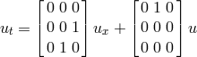
For simplicity we consider the wave equation in 1+1 dimensions. Choosing Cartesian coordinates we have,

ϕtt − ϕxx = 0,

and so defining the “vector” $u := (ϕ,ϕt,ϕx )$ we have the following first order system:

⌊ ⌋ ⌊ ⌋ 0 0 0 0 1 0 ut = |⌈0 0 1|⌉ ux + |⌈ 0 0 0 |⌉u 0 1 0 0 0 0

There are several other notions of hyperbolicity that appear in the literature:

A first order system is called weakly hyperbolic if the eigenvalues of the principal part are purely imaginary. This condition, clearly weaker than strong hyperbolicity, is not enough to assert well posedness in the sense I have defined here, and so I do not discuss it further.
A first order system is called strictly hyperbolic if all eigenvalues of the principal part are purely imaginary and distinct. If the eigenvalues are distinct, then the eigenspaces invariant under the action of $P1(iω)$ are one dimensional and the system can be diagonalized. Thus this class is contained in the strongly hyperbolic one. Due to the degeneracies of systems induced by symmetries in more than one dimension, physical problems are seldom strictly hyperbolic. Sometimes this definition is used to mean that the eigenvectors belonging to the different invariant spaces generated by the symmetries, which must be also invariant under $iAa ωa$ , have distinct eigenvalues. With suitable conditions on the symmetries, this implies the full diagonalization of the principal part, and so equivalence with strong hyperbolicity.
There is a slightly different notion of hyperbolicity due to Leray see [50 ] and [51 ]. There a system is called strictly hyperbolic, or just hyperbolic, if it satisfies certain conditions which amount to having the Cauchy problem well posed in the sense we have used. A system is called non-strictly hyperbolic if it satisfies conditions implying well posedness of the Cauchy Problem, but where the continuity notion is not given by a norm, but rather through Gevrey classes of functions. In particular these spaces are subspaces of smooth, $∞ C$ functions, and so the data must be also smooth. I doubt very much can be done with them in terms of studying the stability of numerical methods, so we shall not concentrate on them.