In this and the following sections we will construct a number of bitensors, tensorial functions of two points
in spacetime. The first is ![]() , to which we refer as the “base point”, and to which we assign indices
, to which we refer as the “base point”, and to which we assign indices ![]() ,
,
![]() , etc. The second is
, etc. The second is ![]() , to which we refer as the “field point”, and to which we assign indices
, to which we refer as the “field point”, and to which we assign indices
![]() ,
, ![]() , etc. We assume that
, etc. We assume that ![]() belongs to
belongs to ![]() , the normal convex neighbourhood of
, the normal convex neighbourhood of
![]() ; this is the set of points that are linked to
; this is the set of points that are linked to ![]() by a unique geodesic. The geodesic
by a unique geodesic. The geodesic ![]() that links
that links ![]() to
to ![]() is described by relations
is described by relations ![]() in which
in which ![]() is an affine parameter
that ranges from
is an affine parameter
that ranges from ![]() to
to ![]() ; we have
; we have ![]() and
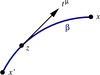
and ![]() . To an arbitrary point
. To an arbitrary point
![]() on the geodesic we assign indices
on the geodesic we assign indices ![]() ,
, ![]() , etc. The vector
, etc. The vector ![]() is tangent to
the geodesic, and it obeys the geodesic equation
is tangent to
the geodesic, and it obeys the geodesic equation ![]() . The situation is illustrated in
Figure 5
. The situation is illustrated in
Figure 5![]() .
.
Synge’s world function is a scalar function of the base point ![]() and the field point
and the field point ![]() . It is defined by
. It is defined by
By virtue of the geodesic equation, the quantity ![]() is constant on the geodesic. The world
function is therefore numerically equal to
is constant on the geodesic. The world
function is therefore numerically equal to ![]() . If the geodesic is timelike, then
. If the geodesic is timelike, then ![]() can be set
equal to the proper time
can be set
equal to the proper time ![]() , which implies that
, which implies that ![]() and
and ![]() . If the geodesic is spacelike,
then
. If the geodesic is spacelike,
then ![]() can be set equal to the proper distance
can be set equal to the proper distance ![]() , which implies that
, which implies that ![]() and
and ![]() . If the
geodesic is null, then
. If the
geodesic is null, then ![]() . Quite generally, therefore, the world function is half the squared geodesic
distance between the points
. Quite generally, therefore, the world function is half the squared geodesic
distance between the points ![]() and
and ![]() .
.
In flat spacetime, the geodesic linking ![]() to
to ![]() is a straight line, and
is a straight line, and ![]() in
Lorentzian coordinates.
in
Lorentzian coordinates.
The world function ![]() can be differentiated with respect to either argument. We let
can be differentiated with respect to either argument. We let ![]() be its partial derivative with respect to
be its partial derivative with respect to ![]() , and
, and ![]() its partial derivative with respect to
its partial derivative with respect to ![]() .
It is clear that
.
It is clear that ![]() behaves as a dual vector with respect to tensorial operations carried out at
behaves as a dual vector with respect to tensorial operations carried out at ![]() , but as
a scalar with respect to operations carried out
, but as
a scalar with respect to operations carried out ![]() . Similarly,
. Similarly, ![]() is a scalar at
is a scalar at ![]() but a dual vector at
but a dual vector at
![]() .
.
We let ![]() be the covariant derivative of
be the covariant derivative of ![]() with respect to
with respect to ![]() ; this is a rank-2
tensor at
; this is a rank-2
tensor at ![]() and a scalar at
and a scalar at ![]() . Because
. Because ![]() is a scalar at
is a scalar at ![]() , we have that this tensor is
symmetric:
, we have that this tensor is
symmetric: ![]() . Similarly, we let
. Similarly, we let ![]() be the partial derivative
of
be the partial derivative
of ![]() with respect to
with respect to ![]() ; this is a dual vector both at
; this is a dual vector both at ![]() and
and ![]() . We can also define
. We can also define
![]() to be the partial derivative of
to be the partial derivative of ![]() with respect to
with respect to ![]() . Because partial
derivatives commute, these bitensors are equal:
. Because partial
derivatives commute, these bitensors are equal: ![]() . Finally, we let
. Finally, we let ![]() be the
covariant derivative of
be the
covariant derivative of ![]() with respect to
with respect to ![]() ; this is a symmetric rank-2 tensor at
; this is a symmetric rank-2 tensor at ![]() and a scalar at
and a scalar at
![]() .
.
The notation is easily extended to any number of derivatives. For example, we let ![]() ,
which is a rank-3 tensor at
,
which is a rank-3 tensor at ![]() and a dual vector at
and a dual vector at ![]() . This bitensor is symmetric in the pair of indices
. This bitensor is symmetric in the pair of indices
![]() and
and ![]() , but not in the pairs
, but not in the pairs ![]() and
and ![]() , nor
, nor ![]() and
and ![]() . Because
. Because ![]() is here an ordinary partial
derivative with respect to
is here an ordinary partial
derivative with respect to ![]() , the bitensor is symmetric in any pair of indices involving
, the bitensor is symmetric in any pair of indices involving ![]() . The ordering
of the primed index relative to the unprimed indices is therefore irrelevant: The same bitensor can be
written as
. The ordering
of the primed index relative to the unprimed indices is therefore irrelevant: The same bitensor can be
written as ![]() or
or ![]() or
or ![]() , making sure that the ordering of the unprimed indices is not
altered.
, making sure that the ordering of the unprimed indices is not
altered.
More generally, we can show that derivatives of any bitensor ![]() satisfy the property
satisfy the property
The message of Equation (54![]() ), when applied to derivatives of the world function, is that while the
ordering of the primed and unprimed indices relative to themselves is important, their ordering with respect
to each other is arbitrary. For example,
), when applied to derivatives of the world function, is that while the
ordering of the primed and unprimed indices relative to themselves is important, their ordering with respect
to each other is arbitrary. For example, ![]() .
.
We can compute ![]() by examining how
by examining how ![]() varies when the field point
varies when the field point ![]() moves. We let the new
field point be
moves. We let the new
field point be ![]() , and
, and ![]() is the corresponding variation of
the world function. We let
is the corresponding variation of
the world function. We let ![]() be the unique geodesic that links
be the unique geodesic that links ![]() to
to ![]() ; it is
described by relations
; it is
described by relations ![]() , in which the affine parameter is scaled in such a way
that it runs from
, in which the affine parameter is scaled in such a way
that it runs from ![]() to
to ![]() also on the new geodesic. We note that
also on the new geodesic. We note that ![]() and
and
![]() .
.
Working to first order in the variations, Equation (53![]() ) implies
) implies
where ![]() , an overdot indicates differentiation with respect to
, an overdot indicates differentiation with respect to ![]() , and the metric and its
derivatives are evaluated on
, and the metric and its
derivatives are evaluated on ![]() . Integrating the first term by parts gives
. Integrating the first term by parts gives
The integral vanishes because ![]() satisfies the geodesic equation. The boundary term at
satisfies the geodesic equation. The boundary term at ![]() is zero because the variation
is zero because the variation ![]() vanishes there. We are left with
vanishes there. We are left with ![]() , or
, or
A virtually identical calculation reveals how ![]() varies under a change of base point
varies under a change of base point ![]() . Here the
variation of the geodesic is such that
. Here the
variation of the geodesic is such that ![]() and
and ![]() , and we obtain
, and we obtain
![]() . This shows that
. This shows that
It is interesting to compute the norm of ![]() . According to Equation (55
. According to Equation (55![]() ) we have
) we have
![]() . According to Equation (53
. According to Equation (53![]() ), this is equal to
), this is equal to ![]() . We have obtained
. We have obtained
We note that in flat spacetime, ![]() and
and ![]() in Lorentzian
coordinates. From this it follows that
in Lorentzian
coordinates. From this it follows that ![]() , and finally,
, and finally,
![]() .
.
If the base point ![]() is kept fixed,
is kept fixed, ![]() can be considered to be an ordinary scalar function of
can be considered to be an ordinary scalar function of ![]() .
According to Equation (57
.
According to Equation (57![]() ), this function is a solution to the nonlinear differential equation
), this function is a solution to the nonlinear differential equation
![]() . Suppose that we are presented with such a scalar field. What can we say about
it?
. Suppose that we are presented with such a scalar field. What can we say about
it?
An additional differentiation of the defining equation reveals that the vector ![]() satisfies
satisfies
The vector
is a normalized tangent vector that satisfies the geodesic equation in affine-parameter form:In the affine parameterization, the expansion of the congruence is calculated to be
where These considerations, which all follow from a postulated relation ![]() , are clearly compatible
with our preceding explicit construction of the world function.
, are clearly compatible
with our preceding explicit construction of the world function.
| http://www.livingreviews.org/lrr-2004-6 |
© Max Planck Society
Problems/comments to |