4.2 Distributions in curved spacetime
The distributions introduced in Section 4.1.5 can also be defined in a four-dimensional spacetime
with metric  . Here we produce the relevant generalizations of the results derived in that
section.
. Here we produce the relevant generalizations of the results derived in that
section.
4.2.1 Invariant Dirac distribution
We first introduce  , an invariant Dirac functional in a four-dimensional curved spacetime. This is
defined by the relations
, an invariant Dirac functional in a four-dimensional curved spacetime. This is
defined by the relations
where  is a smooth test function,
  any four-dimensional region that contains
  , and
, and  any
four-dimensional region that contains
any
four-dimensional region that contains  . These relations imply that
  is symmetric in its
arguments, and it is easy to see that
where
is symmetric in its
arguments, and it is easy to see that
where  is the ordinary (coordinate)
four-dimensional Dirac functional. The relations of Equation (259) are all equivalent because
is the ordinary (coordinate)
four-dimensional Dirac functional. The relations of Equation (259) are all equivalent because
 is a distributional identity; the last form is manifestly symmetric in
  and
and
 .
.
The invariant Dirac distribution satisfies the identities
where  is any bitensor and
  ,
,  are parallel propagators. The first identity
follows immediately from the definition of the
are parallel propagators. The first identity
follows immediately from the definition of the  -function. The second and third identities are established
by showing that integration against a test function
-function. The second and third identities are established
by showing that integration against a test function  gives the same result from both sides. For
example, the first of the Equations (258) implies
gives the same result from both sides. For
example, the first of the Equations (258) implies
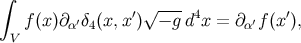
and on the other hand,
![∫ ∮ α ′ √ --- 4 α ′ α ′ − f(x )(g α′δ4(x,x ));α − g d x = − f (x)g α′δ4(x,x )dΣ α + [f,αg α′] = ∂α′f(x ), V ∂V](article1989x.gif)
which establishes the second identity of Equation (260). Notice that in these manipulations, the
integrations involve scalar functions of the coordinates  ; the fact that these functions are also vectors
with respect to
; the fact that these functions are also vectors
with respect to  does not invalidate the procedure. The third identity of Equation (260) is proved in a
similar way.
does not invalidate the procedure. The third identity of Equation (260) is proved in a
similar way.
4.2.2 Light-cone distributions
For the remainder of Section 4.2 we assume that  , so that a unique geodesic
  links these two
points. We then let
links these two
points. We then let  be the curved spacetime world function, and we define light-cone step
functions by
be the curved spacetime world function, and we define light-cone step
functions by
where  is one if
  is in the future of the spacelike hypersurface
  and zero otherwise, and
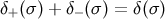
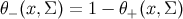 . These are immediate generalizations to curved spacetime of the objects
defined in flat spacetime by Equation (246). We have that
. These are immediate generalizations to curved spacetime of the objects
defined in flat spacetime by Equation (246). We have that  is one if
  is an element
of
is an element
of  , the chronological future of
  , and zero otherwise, and
  is one if
  is an element of
  , the chronological past of
  , and zero otherwise. We also have
 .
.
We define the curved-spacetime version of the light-cone Dirac functionals by
an immediate generalization of Equation (247). We have that  , when viewed as a function of
  , is
supported on the future light cone of
, is
supported on the future light cone of  , while
  is supported on its past light cone. We also have
 , and we recall that
  is negative if
  and
and  are timelike related, and positive
if they are spacelike related.
are timelike related, and positive
if they are spacelike related.
For the same reasons as those mentioned in Section 4.1.5, it is sometimes convenient to shift the
argument of the step and  -functions from
  to
to  , where
  is a small positive quantity. With
this shift, the light-cone distributions can be straightforwardly differentiated with respect to
is a small positive quantity. With
this shift, the light-cone distributions can be straightforwardly differentiated with respect to  . For
example,
. For
example,  , with a prime indicating differentiation with respect to
 .
.
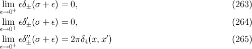
We now prove that the identities of Equation (248, 249, 250) generalize to
in a four-dimensional curved spacetime; the only differences lie with the definition of the world function and
the fact that it is the invariant Dirac functional that appears in Equation (265). To establish these
identities in curved spacetime we use the fact that they hold in flat spacetime – as was shown in
Section 4.1.5 – and that they are scalar relations that must be valid in any coordinate system if they are
found to hold in one. Let us then examine Equations (263, 264) in the Riemann normal coordinates of
Section 3.1; these are denoted  and are based at
  . We have that
  and
and
 , where
  is the van Vleck determinant, whose
coincidence limit is unity. In Riemann normal coordinates, therefore, Equations (263, 264, 265)
take exactly the same form as Equations (248, 264, 250). Because the identities are true in
flat spacetime, they must be true also in curved spacetime (in Riemann normal coordinates
based at
is the van Vleck determinant, whose
coincidence limit is unity. In Riemann normal coordinates, therefore, Equations (263, 264, 265)
take exactly the same form as Equations (248, 264, 250). Because the identities are true in
flat spacetime, they must be true also in curved spacetime (in Riemann normal coordinates
based at  ); and because these are scalar relations, they must be valid in any coordinate
system.
); and because these are scalar relations, they must be valid in any coordinate
system.
![Ω...(x,x′)δ4(x, x′) = [Ω...]δ4(x,x′), ( ′ ) (260 ) (gαα′(x,x ′)δ4(x,x′));α = − ∂α′δ4(x, x′), gαα(x′,x)δ4(x, x′);α′= − ∂αδ4(x,x′),](article1982x.gif)