Formalism

6 Formalism

I give here a simple technical description of the formalism of loop quantum gravity. For a more detailed construction, see [261

, 294

, 292 , 33 ].

6.1 Classical theory

The starting point of the construction of quantum theory is classical general relativity, formulated in terms of the Sen–Ashtekar–Barbero connection [271 , 16 , 61 ]. Detailed introductions to the (complex) Ashtekar formalism can be found in the book [18 ] and in the conference proceedings [103 ]. The real version of the theory is presently the most widely used.

Classical general relativity can be formulated in phase-space form as follows [18 , 61 ]. Fix a three-dimensional manifold $M$ (compact and without boundaries) and consider a smooth real $SU (2)$ connection $Aia(x)$ and a vector density $&tidle;Eai (x)$ , transforming in the vector representation of $SU (2)$ on $M$ . We use $a,b,...= 1,2, 3$ for spatial indices and $i,j,...= 1,2,3$ for internal indices. The internal indices can be viewed as labeling a basis in the Lie algebra of $SU (2)$ or the three axis of a local triad. We indicate coordinates on $M$ as $x$ . The relation between these fields and conventional metric gravitational variables is as follows: $E&tidle;ai (x)$ is the (densitized) inverse triad, related to the three-dimensional metric $gab(x)$ of constant-time surfaces by

where $g$ is the determinant of $gab$ ; and

$Γ i(x ) a$ is the spin connection associated to the triad. (This is defined by $∂ ei = Γ ie [a b] [a b]j$ , where $ei a$ is the triad). $i ka(x)$ is the extrinsic curvature of the constant-time three-surface.

In Equation (2 ), $γ$ is a constant, denoted the Immirzi parameter, that can be chosen arbitrarily (it will enter the Hamiltonian constraint) [152 , 151 , 150 ]. Different choices for $γ$ yield different versions of the formalism, all equivalent in the classical domain. If we choose $γ$ to be equal to the imaginary unit, $√ --- γ = − 1$ , then $A$ is the standard Ashtekar connection, which can be shown to be the projection of the self-dual part of the four-dimensional spin connection on the constant-time surface. If we choose $γ = 1$ , we obtain the real Barbero connection. The Hamiltonian constraint of Lorentzian general relativity has a particularly simple form in the $γ = √−-1$ formalism; while the Hamiltonian constraint of Euclidean general relativity has a simple form when expressed in terms of the $γ = 1$ real connection. Other choices of $γ$ are viable as well. Different choices of $γ$ are genuinely physical physically? nonequivalent in the quantum theory, since they yield “geometrical quanta” of different magnitude [270 ]. It has been argued that there is a unique choice of $γ$ yielding the correct $1∕4$ coefficient in the Bekenstein–Hawking formula [170 , 171 , 253 , 22 , 254 , 92 ], but the matter is still under discussion; see for instance [160 ].

The spinorial version of the Ashtekar variables is given in terms of the Pauli matrices $σi,i = 1,2,3$ , or the $SU (2)$ generators $τi = − i2 σi$ , by

&tidle;a &tidle;a &tidle;a E (x) = − iE i (x)σi = 2E i (x)τi, (3 ) i- i i Aa (x) = − 2 A a(x)σi = A a(x)τi. (4 )

Thus, $Aa(x)$ and $&tidle;a E (x)$ are $2 × 2$ anti-Hermitian complex matrices.

The theory is invariant under local $SU (2 )$ gauge transformations, three-dimensional diffeomorphisms of the manifold on which the fields are defined, as well as under (coordinate) time translations generated by the Hamiltonian constraint. The full dynamical content of general relativity is captured by the three constraints that generate these gauge invariances.

The Lorentzian Hamiltonian constraint does not have a simple polynomial form if we use the real connection (2 ). For a while, this fact was considered an obstacle to defining the quantum Hamiltonian constraint; therefore, the complex version of the connection was mostly used. However, Thiemann has succeeded in constructing a Lorentzian quantum-Hamiltonian constraint [285 , 289 , 291 ] in spite of the non-polynomiality of the classical expression. This is why the real connection is now widely used. This choice has the advantage of eliminating the old “reality conditions” problem, namely the problem of implementing nontrivial reality conditions in the quantum theory.

Alternative versions of the classical formalism used as a starting point for the quantization have been explored in the literature. Of particular interest is the approach followed by Alexandrov, who has argued for a formalism where the full local $SO (3, 1)$ symmetry of the tetrad formalism is manifestly maintained [4 , 5 , 6 ]. One of the advantages of this approach is that it sheds light on the relationship with covariant spin-foam formalism (see below). Its main difficulty is to fully keep track of the complicated second-class constraints and the resulting nontrivial Dirac algebra.

6.2 Quantum kinematics

Certain classical quantities play a very important role in the quantum theory. These are: traces of the holonomy of the connection, which are labeled by loops on the 3-manifold; and surface integrals of the triad. Given a loop $α$ in $M$ define:

where $Uα ∼ 𝒫exp {∮ A } α$ is the parallel propagator of $Aa$ along $α$ , which is defined by $Uα(0) = 11$ ,

and $Uα = U α(1)$ . Given a two-dimensional surface $S$ , define

where $f$ is a function on the surface $S$ , taking values in the Lie algebra of $SU (2)$ . These two quantities are naturally represented as quantum operators on the Hilbert space of the quantum theory, which I now define.

Consider a “Schrödinger-like” representation formed by quantum states that are functionals $ψ (A)$ of the connection. On these states, the two quantities $𝒯 [α ]$ and $E[S,f ]$ act naturally: the first as a multiplicative operator, the second as the functional derivative operator

This defines an heuristic quantization, à la Wheeler–DeWitt. What is needed to make it mathematically precise, and to make it usable for concrete calculations is a precise characterization of the class of functionals $ψ(A )$ to be considered, and, especially, a definition of the scalar product among these. Let us do so.

The class of functionals that we will use is formed by (the closure in the Hilbert-space norm of the linear span of) functionals of a particular class, denoted “cylindrical states”. These are defined as follows. Pick a graph $Γ$ , say with $n$ links, denoted $γ ...γ 1 n$ , immersed in the manifold $M$ . Let $Ui(A ) = Uγi, i = 1, ...,n$ be the parallel transport operator of the connection $A$ along $γi$ . $Ui(A )$ is an element of $SU (2)$ . Pick a function $f (g1...gn)$ on $n [SU (2)]$ . The graph $Γ$ and the function $f$ determine a functional of the connection as follows

(These states are called cylindrical states because they were introduced in [28

, 29

, 30

] as cylindrical functions for the definition of a cylindrical measure.) Notice that we can always “enlarge the graph”, in the sense that if $Γ$ is a subgraph of $Γ ′$ , we can always write

by simply choosing $f′$ independent from the $Ui$ ’s of the links, which are in $Γ ′$ but not in $Γ$ . Thus, given any two cylindrical functions, we can always view them as having the same graph (formed by the union of the two graphs). Given this observation, we define the scalar product between any two cylindrical functions [173 , 28

, 29

, 30

] by

where $dg$ is the Haar measure on $SU (2)$ . This scalar product extends by linearity to finite linear combinations of cylindrical functions. It is not difficult to show that Equation (11

) defines a well-defined scalar product on the space of these linear combinations. Completing the space of these linear combinations in the Hilbert norm, we obtain a Hilbert space $ℋ$ . This is the (unconstrained) quantum-state space of loop gravity.

The main property of $ℋ$ is that it carries a natural unitary representation of the diffeomorphism group and of the group of the local $SU (2)$ transformations, obtained transforming the argument of the functionals. In fact, the essential property of the scalar product (11 ) is that it is invariant under both these transformations. The operators $𝒯 [α]$ and $E [S,f]$ are well-defined self-adjoint operators in this Hilbert space.

A number of observations are in order.

The construction of this quantum representation may seem arbitrary, but a powerful theorem [176 , 111 , 112 ], called the LOST theorem (from the initials of the authors of one of the two versions of the theorem), states that, under rather general assumptions, this representation is unique, up to unitary equivalence. This is in the same sense in which the usual Schrödinger representation of nonrelativistic quantum mechanics is unique. The main hypothesis of the theorem is the diffeomorphism invariance of the theory. This shows that diffeomorphism invariance is a powerful constraint on the form of the quantum field theory.
$ℋ$ is nonseparable. After factoring away diffeomorphism invariance, we obtain a separable Hilbert space (see Section 6.4).
From the point of view of the physical intuition, cylindrical functions can be seen first of all as a convenient way to span the space of the functional of the connection. (In a suitable topology, any functional of the connection can be approximated by a linear combination of such functions.) On the other hand, the choice reflects the physics. In Yang–Mills theory, this choice would lead to an inconsistent theory based on a nonseparable Hilbert space. Here, on the other hand, diffeomorphism invariance cures the nonseparability. This is the mathematical implementation of the physical argument concerning the existence of the continuous limit of loop states, which was given in Section 5.2.
Standard spectral theory holds on $ℋ$ , and it turns out that using spin networks (discussed below) one can express $ℋ$ as a direct sum over finite-dimensional subspaces, which have the structure of Hilbert spaces of spin systems; this makes practical calculations very manageable.

Using Dirac notation, we write

in the same manner in which one may write $ψ(x ) = ⟨x |Ψ ⟩$ in ordinary quantum mechanics. As in that case, $|A ⟩$ is not a normalizable state.

6.3 Loop and spin network states

A subspace $ℋ0$ of $ℋ$ is formed by states invariant under $SU (2)$ gauge transformations. We now define an orthonormal basis in $ℋ0$ . This basis represents a very important tool for using the theory. It was introduced in [269 ] and developed in [47 , 48 ]; it is denoted ’spin network basis’.

First, given a loop $α$ in $M$ , there is a normalized state $ψα(A )$ in $ℋ$ , which is obtained by taking $Γ = α$ and $f (g) = − T r(g)$ . Namely

We introduce Dirac notation for the abstract states, and denote this state as $|α ⟩$ . These states are called loop states. Using Dirac notation, we can write

It is easy to show that loop states are normalizable. Products of loop states are normalizable as well. Following tradition, we also denote with $α$ a multiloop, namely a collection of (possibly overlapping) loops ${α1, ...,αn,}$ , and we call

a multiloop state. (Multi-)loop states represented the main tool for loop quantum gravity before the discovery of the spin network basis. Linear combinations of multiloop states (over-)span $ℋ$ , and, therefore, a generic state $ψ (A )$ is fully characterized by its projections on the multiloop states, namely by

The “old” loop representation was based on representing quantum states in this manner, namely by means of the functionals $ψ(α )$ over loop space defined in Equation (16

). Equation (16

) can be explicitly written as an integral transform, as we will see in Section 6.5.

Next, consider a graph $Γ$ . A “coloring” of $Γ$ is given by the following.

Associate an irreducible representation of $SU (2)$ to each link of $Γ$ . Equivalently, associate to each link $γ i$ a half-integer number $j i$ , the spin of the irreducible representation.
Associate an invariant tensor $v$ in the tensor product of the representations $j1 ...jn$ to each node of $Γ$ in which links with spins $j1 ...jn$ meet. An invariant tensor is an object with $n$ indices in the representations $j1 ...jn$ that transform covariantly. If $n = 3$ , there is only one invariant tensor (up to a multiplicative factor), given by the Clebsch–Gordan coefficient. An invariant tensor is also called an intertwiner. All intertwiners are given by the standard Clebsch–Gordan theory. More precisely, for fixed $j1 ...jn$ , the invariant tensors form a finite-dimensional linear space. Pick a basis $vi$ is this space, and associate one of these basis elements to the node. Notice that invariant tensors exist only if the tensor product of the representations $j1...jn$ contains the trivial representation. This yields a condition on the coloring of the links. For $n = 3$ , this is given by the well -known Clebsch-Gordan condition: each color is not larger than the sum of the other two, and the sum of the three colors is even.

Indicate a colored graph by ${Γ ,⃗j,⃗v}$ , or simply $S = {Γ ,⃗j,⃗v}$ , and denote it a “spin network”. (It was Penrose who first had the intuition that this mathematics could be relevant for describing the quantum properties of the geometry, and who gave the first version of spin-network theory [223 , 224 ].)

Given a spin network $S$ , we can construct a state $ΨS (A)$ as follows. Take the propagator of the connection along each link of the graph in the representation associated to that link, and then, at each node, contract the matrices of the representation with the invariant tensor. We obtain a state $ΨS (A )$ , which we also write as

One can then show the following.

The spin network states are normalizable.
They are $SU (2 )$ gauge invariant.
Each spin network state can be decomposed into a finite linear combination of products of loop states.
The (normalized) spin network states form an orthonormal basis for the gauge $SU (2)$ invariant states in $ℋ$ (choosing the basis of invariant tensors appropriately).

The spin network states provide a very convenient basis for the quantum theory, with a direct physical interpretation. This follows from the fact that the spin network states are eigenstates of area and volume operators, therefore they are states in which the three-dimensional geometry is well defined. See [261 ] for details.

Consider the relations between the loop states

and the states $ψ(A )$ giving the amplitude for a connection field configuration $A$ , and defined by

Here $|A ⟩$ are “eigenstates of the connection operator”, or, more precisely (since the operator corresponding to the connection is ill defined in the theory), the generalized states that satisfy

We can write, for every spin network $S$ , and every state $ψ (A )$

This equation defines a unitary mapping between the two presentations of $ℋ$ : the “loop representation”, in which one works in terms of the basis $|S⟩$ ; and the “connection representation”, in which one uses wave functionals $ψ(A )$ .

6.4 Diffeomorphism invariance

The next step in the construction of the theory is to factor away diffeomorphism invariance. This is a key step for two reasons. First of all, $ℋ$ is a “huge” nonseparable space. It is far “too large” for a quantum field theory. However, most of this redundancy is gauge, and disappears when one solves the diffeomorphism constraint, defining the diff-invariant Hilbert space $ℋDiff$ . This is the reason for which the loop representation, as defined here, is only of value in diffeomorphism invariant theories.

The second reason is that $ℋDiff$ turns out to have a natural basis labeled by knots. More precisely by “s-knots”. An s-knot s is an equivalence class of spin networks S under diffeomorphisms. An s-knot is characterized by its “abstract” graph (defined only by the adjacency relations between links and nodes), by the coloring, and by its knotting and linking properties, as in knot theory. Thus, the physical quantum states of the gravitational field turn out to be essentially classified by knot theory.

There are various equivalent ways of obtaining $ℋDiff$ from $ℋ$ . One can use regularization techniques for defining the quantum operator corresponding to the classical diffeomorphism constraint in terms of elementary loop operators, and then find the kernel of such operator. Equivalently, one can factor $ℋ$ by the natural action of the diffeomorphism group that it carries. Namely

There are several rigorous ways for defining the quotient of a Hilbert space by the unitary action of a group. See in particular the construction in [34 ], which follows the ideas of Marolf and Higuchi [194 , 196 , 197 , 145 ].

In the quantum gravity literature, a big deal has been made of the problem that a scalar product is not defined on the space of solutions of a constraint $ˆC$ , defined on a Hilbert space $ℋ$ . This, however, is a false problem. It is true that if zero is in the continuum spectrum of $ˆC$ , then the corresponding eigenstates are generalized states and the $ℋ$ scalar product is not defined between them. But the generalized eigenspaces of $ˆ C$ , including the kernel, nevertheless inherit a scalar product from $ˆ H$ . This can be seen in a variety of equivalent ways. For instance, it can be seen from the following theorem. If $Cˆ$ is self-adjoint, then there exists a measure $μ(λ )$ on its spectrum and a family of Hilbert spaces $ℋ (λ)$ such that

where the integral is the continuous sum of Hilbert spaces described, for instance, in [138 ]. Clearly $ℋ (0)$ is the kernel of $ˆ C$ equipped with a scalar product. This is discussed, for instance, in [239 ].

When factoring away the diffeomorphisms in the quantum-theory finite-dimensional moduli spaces associated with high valence, nodes appear [137 ]. Because of these, the resulting Hilbert space is still nonseparable. These moduli parameters, however, have no physical significance and do not play any role in the quantum theory. They can be discarded by judicious choice of the functional space in which the fields are defined [110 , 299 , 300 ], or in other ways [294 ].

6.5 Other structures in $ℋ$

The mathematical foundations of loop quantum gravity have been developed to the level of rigor of mathematical physics. This has introduced some heavy mathematical tools, sometimes unfamiliar to the average physicist, at the price of widening the language gap between scientists who study quantum gravity and other parts of the community. There is good reason for seeking a mathematical-physics level of precision in quantum gravity. In the development of conventional quantum field theory mathematical rigor could be low because extremely accurate empirical verifications assured physicists that “the theory may be mathematically meaningless, but it is nevertheless physically correct, and therefore the theory must make sense, even if we do not understand well how.” In quantum gravity this indirect experimental reassurance is lacking and the claim that the theory is well founded can be based only on a solid mathematical control. Given the unlikelihood of finding direct experimental corroboration, the research can only aim for the moment at the goal of finding a consistent theory, with correct limits in the regimes that we control experimentally. High mathematical rigor is the only assurance of the consistency of the theory. Quantum field theory on manifolds is an unfamiliar terrain in which the experience accumulated in conventional quantum field theory is often useless and sometimes misleading.

One may object that a rigorous definition of quantum gravity is a vain hope, given that we do not even have a rigorous definition of QED, presumably a much simpler theory. The objection is particularly valid from the point of view of a physicist who views gravity “just as any other field theory; like the ones we already understand”. But the (serious) difficulties of QED and of other conventional field theories are ultraviolet. The physical hope supporting the quantum gravity research program is that the ultraviolet structure of a diffeomorphism-invariant quantum field theory is profoundly different from the one of conventional theories. Indeed, recall that in a very precise sense there is no short distance limit in the theory; the theory naturally cuts itself off at the Planck scale, due to the very quantum discreteness of spacetime. Thus, the hope that quantum gravity could be defined rigorously may be optimistic, but it is not ill founded.

After these comments, let me briefly mention some of the structures that have been explored in $ℋ$ . First of all, the spin-network states satisfy the Kauffman axioms of the tangle theoretical version of recoupling theory [162 ] (in the “classical” case $A = − 1$ ) at all the points (in 3D space) where they meet. For instance, consider a 4-valent node of four links colored $a,b,c,d$ . The color of the node is determined by expanding the 4-valent node into a trivalent tree; in this case, we have a single internal link. The expansion can be done in different ways (by pairing links differently). These are related to each other by the recoupling theorem of pg. 60 in Ref. [162 ]

where the quantities ${ } a b i c d j$ are $SU (2)$ six-j symbols (normalized as in [162

]). Equation (24

) follows just from the definitions given above. Recoupling theory provides a powerful computational tool in this context (see [298 , 77 , 88 ]).

Since spin network states satisfy recoupling theory, they form a Temperley–Lieb algebra [162 ]. The scalar product (11 ) in $ℋ$ is also given by the Temperley–Lieb trace of the spin networks, or, equivalently by the Kauffman brackets, or, equivalently, by the chromatic evaluation of the spin network.

Next, $ℋ$ admits a rigorous representation as an $L2$ space, namely a space of square-integrable functions. To obtain this representation, however, we have to extend the notion of connection, to a notion of “distributional connection”. The space of the distributional connections is the closure of the space of smooth connection in a certain topology. Thus, distributional connections can be seen as limits of sequences of connections, in the same manner in which distributions can be seen as limits of sequences of functions. Usual distributions are defined as elements of the topological dual of certain spaces of functions. Here, there is no natural linear structure in the space of the connections, but there is a natural duality between connections and curves in $M$ : a smooth connection $A$ assigns a group element $U γ(A )$ to every segment $γ$ . The group elements satisfy certain properties. For instance if $γ$ is the composition of the two segments $γ1$ and $γ2$ , then $U (A) = U (A )U (A ) γ γ1 γ2$ .

A generalized connection $¯ A$ is defined as a map that assigns an element of $SU (2)$ , which we denote as $U γ(A ¯)$ or $¯A(γ)$ , to each (oriented) curve $γ$ in $M$ , satisfying the following requirements: i) $A¯(γ−1) = (A¯(γ))−1$ ; and ii) $A¯(γ2 ∘ γ1) = A¯(γ2) ⋅A¯(γ1)$ , where $γ−1$ is obtained from $γ$ by reversing its orientation, $γ2 ∘ γ1$ denotes the composition of the two curves (obtained by connecting the end of $γ1$ with the beginning of $γ2$ ) and $¯ ¯ A (γ2) ⋅A (γ1)$ is the composition in $SU (2)$ . The space of such generalized connections is denoted $-- 𝒜$ . The cylindrical functions $Ψ Γ ,f(A )$ , defined in Section 6.3 as functions on the space of smooth connections, extend immediately to generalized connections

We can define a measure $dμ0$ on the space of generalized connections $-- 𝒜$ by

In fact, one may show that Equation (26

) defines (by linearity and continuity) a well-defined absolutely-continuous measure on $-- 𝒜$ . This is the Ashtekar–Lewandowski (or Ashtekar–Lewandowski–Baez) measure [28 , 29 , 30 , 45 ]. Then, one can prove that $-- ℋ = L2[𝒜, dμ0]$ under the natural isomorphism given by identifying cylindrical functions. It follows immediately that the transformation (16

) between the connection representation and the “old” loop representation is given by

This is the loop transform formula [265 ]; here it becomes rigorously defined.

Furthermore, $ℋ$ can be seen as the projective limit of the projective family of the Hilbert spaces $ℋ Γ$ , associated to each graph $Γ$ immersed in $M$ . $ℋ Γ$ is defined as the space $n L2 [SU (2 ) ,dg1...dgn]$ , where $n$ is the number of links in $Γ$ . The cylindrical function $Ψ Γ ,f(A )$ is naturally associated to the function $f$ in $ℋ Γ$ , and the projective structure is given by the natural map (10 ) [34 , 198 ].

Finally, Ashtekar and Isham [27 ] have recovered the representation of the loop algebra by using C*-algebra representation theory: the space $𝒜-∕𝒢$ , where $𝒢$ is the group of local $SU (2)$ transformations (which acts in the obvious way on generalized connections), is precisely the Gelfand spectrum of the Abelian part of the loop algebra. One can show that this is a suitable norm closure of the space of smooth $SU (2)$ connections over physical space, modulo gauge transformations.

Thus, a number of powerful mathematical tools are at hand for dealing with nonperturbative quantum gravity. These include Penrose’s spin network theory, $SU (2)$ representation theory, Kauffman tangle theoretical recoupling theory, Temperley–Lieb algebras, Gelfand’s $C ∗$ algebra, spectral-representation theory, infinite-dimensional measure theory and differential geometry over infinite-dimensional spaces.

6.6 Dynamics: I. Hamiltonian

The definition of the theory is completed by giving the Hamiltonian constraint. A number of approaches to the definition of a Hamiltonian constraint have been attempted in the past, with various degrees of success. Thiemann has succeeded in providing a regularization of the Hamiltonian constraint that yields a well-defined, finite operator. Thiemann’s construction [285 , 289 , 291 ] is based on several clever ideas. I will not describe it here. Rather, I will sketch below in a simple manner the final form of the constraint (for the Lapse = 1 case), following [252 ]. For a complete treatment, see [294 ].

I begin with the Euclidean Hamiltonian constraint. We have

Here $i$ labels the nodes of the s-knot s; $(IJ )$ labels couples of (distinct) links emerging from $i$ . $j1...jn$ are the spins of the links emerging from $i$ . $ˆDi;(IJ)εε′$ is the operator that acts on an s-knot by: (i) creating two additional nodes, one along each of the two links $I$ and $J$ , (ii) creating a novel link, colored $1 2$ , joining these two nodes, (iii) assigning the coloring $jI + ε$ and, respectively, $′ jJ + ε$ to the links that join the new formed nodes with the node $i$ . This is illustrated in Figure 2

Figure 2:

Action of $ˆDi;(IJ)εε′$ .

The coefficients $A εε′(ji...jn)$ , which are finite, can be expressed explicitly (but in a rather laborious way) in terms of products of linear combinations of Wigner 6 $j$ symbols of $SU (2)$ . The Lorentzian Hamiltonian constraint is given by a similar expression, but quadratic in the $ˆD$ operators.

The operator defined above is obtained by introducing a regularized expression for the classical Hamiltonian constraint, written in terms of elementary loop observables, turning these observables into the corresponding operators and taking the limit. The construction works rather magically, relying on the fact [267 ] that certain operator limits $ˆO δ → δ→0 Oˆ$ turn out to be finite on diff-invariant states, thanks to the fact that, for $δ$ and $δ′$ sufficiently small, $Oˆ |Ψ ⟩ δ$ and $ˆ O δ′|Ψ ⟩$ are diffeomorphic equivalent. Thus, here diff invariance plays again the crucial role in the theory.

During the last years, Thomas Thiemann has introduced the idea of replacing the full set of quantum constraints with a single (“master”) constraint [293 ]. The development of this formulation of the dynamics is in progress.

6.7 Dynamics: II. Spin foams

Alternatively, the dynamics of the spin-network states can be defined via the spin-foam formalism. This is a covariant, rather than canonical, language, which can be used to define the dynamics of loop quantum gravity, in the same sense in which giving the covariant vertex amplitude defines the dynamics of the photon and electron states.

In three dimensions, the spin-foam formalism gives the well-known Ponzano–Regge model. Here the vertex amplitude turns out to be given by an $SU (2)$ Wigner 6 $j$ symbol. The relation between this model and loop quantum gravity has been pointed out long ago [248 ], and the complete equivalence has been proven by Alejandro Perez and Karim Noui [210 ].

In four dimensions, an important role has been been played by the Barrett–Crane model, a much-studied spin-foam theory constructed [97 , 221 ] from the definition of the vertex as an $SU (2 )$ Wigner 10 $j$ symbol, given by Louis Crane and John Barrett in [66 ]. There are several difficulties in using the Barrett–Crane model for defining the dynamics of 4D loop quantum gravity [53 , 52 ]. First, the Barrett–Crane model is formulated keeping local Lorentz invariance manifest, while loop quantum gravity is not. This problem has been investigated by Sergei Alexandrov, see [4 , 5 , 7 ] and references therein. Second, the Barrett–Crane model appears to have fewer degrees of freedom than general relativity on a spacelike surface, because it fixes the values of the intertwiners. More importantly, the low-energy limit of the propagator defined by the Barrett–Crane model does not seem to be correct [2 , 3 ]. An important recent development, however, has been the introduction of a new vertex amplitude, defined by the square of the $SU (2)$ Wigner 15 $j$ symbol, which may correct all these problems [106 ]. This has given rise to a rapid development [105 , 181 , 182 , 227 ] and formulation of a class of spin-foam models that may provide a viable definition of the LQG dynamics [104 , 114 , 6 ], and are currently under intense investigation. Some preliminary results appear to be encouraging [188 ].

What characterizes the spin-foam formalism is the fact that it can be derived in a surprising variety of different ways, which all converge to essentially the same structure. The formalism can be obtained (i) from loop gravity, (ii) as a quantization of a discretization of general relativity on a simplicial triangulation, (iii) as a generalization of matrix models to higher dimensions, (iv) from a quantization of the elementary geometry of tetrahedra and 4-simplices, and (v) by quantizing general relativity from its formulation as a constrained BF theory, by imposing constraints on quantum topological theory. Each of these derivations sheds some light on the formalism. For detailed introductions to the spin-foam formalism see [50 , 229 , 230 , 212 , 64 , 177 ]. A recent derivation as the quantization of a discretization of general relativity is in [105 , 104 ], which can also be seen as an independent derivation of the loop-gravity canonical formalism itself. The PhD thesis of Daniele Oriti [213 ] is also a very good introduction. Here I give only a simple heuristic description of the way spin foams appear from loop gravity.

In his PhD thesis, Feynman introduced a path-integral formulation of quantum mechanics, deriving it from the canonical formalism. He considered a perturbation expansion for the matrix elements of the evolution operator

One can search for a covariant formulation of loop quantum gravity following the same idea [257 , 236 ]. The matrix elements of the operator $U (T)$ obtained exponentiating the (Euclidean) Hamiltonian constraint in the proper-time gauge (the operator that generates evolution in proper time) can be expanded in a Feynman sum over paths. In conventional QFT each term of a Feynman sum corresponds naturally to a certain Feynman diagram, namely a set of lines in spacetime meeting at vertices (branching points). A similar structure of the terms appears in quantum gravity, if one uses the spin-network basis, but the diagrams are now given by surfaces is spacetime that branch along edges, which in turn meet at vertices.

This is a consequence of the fact that the Hamiltonian operators acts only on nodes. The histories of s-knots (abstract spin networks), evolving under such an action, are branched surfaces, which carry spins on the faces (swept by the links of the spin network) and intertwiners on the edges (swept by the nodes of the spin network). These have been called “spin foams” by John Baez [48 ], who has studied the general structure of theories defined in this manner [49 , 50 ].

Thus, the time evolution of a spin network, which generates spacetime, is given by a spin foam. The spin foam describes the evolving gravitational degrees of freedom. The formulation is “topological” in the sense that one must sum over topologically-nonequivalent surfaces only, and the contribution of each surface depends on its topology only. This contribution is given by the product of the amplitude of the elementary “vertices”, namely points where the edges branch.

Figure 3:

The elementary vertex.

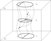
The physical transition amplitude between two s-knot states $|si⟩$ and $|sf ⟩$ turns out to be given by summing over all (branching, colored) surfaces $σ$ that are bounded by the two s-knots $si$ and $sf$

The weight $𝒜 [σ ](T )$ of the spin foam $σ$ is given by a product over the $n$ vertices $v$ of $σ$ :

The contribution $Av (σ )$ of each vertex is given by the matrix elements of the Hamiltonian constraint operator between the two s-knots obtained by slicing $σ$ immediately below and immediately above the vertex. They turn out to depend only on the colors of the surface components immediately adjacent the vertex $v$ . The sum turns out to be finite and explicitly computable order by order.

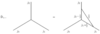
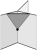
As in the usual Feynman diagrams, the vertices describe the elementary interactions of the theory. Here, in particular, one sees that the complicated structure of the Thiemann Hamiltonian, which makes a node split into three nodes, corresponds to a geometrically very simple vertex. Figure 3 is a picture of the elementary vertex. Notice that it represents nothing but the spacetime evolution of the elementary action of the Hamiltonian constraint, given in Figure 2 . An example of a surface in the sum is given in Figure 4 .

The resulting form of the covariant formulation of quantum gravity as a sum over spin-foam amplitudes is quite different from that of background-dependent quantum field theory.

Spin foams have a very nice geometric interpretation as the dual to a simplicial decomposition of spacetime. Vertices corresponding to four-volumes, edges to three-volumes, etc. This last point is a very elegant feature, and has an immediately intuitive explanation in terms of loop quantum gravity operators. The area operator counts lines in a spin network, corresponding to faces in a spin foam; the volume operator counts vertices in a spin network, corresponding to lines in a spin foam.

Finiteness of some spin-foam models at all orders of perturbation theory has been proven [228 , 94 , 93 ].

Figure 4:

A term of second order.

6.8 Dynamics: III. Group field theory

Very strictly related to the spin-foam language is an intriguing formalism that has been developing in recent years: group field theory. This has emerged from dual formulations of topological theories [76 ], and can be seen as a higher-dimensional version of the duality between matrix models and fluctuating geometries in 2D. Group field theories are standard quantum field theories defined over a group manifold, characterized by a peculiar nonlocal interaction term. They have a remarkable property: the Feynman expansion generates a sum over Feynman graphs that have a direct interpretation as a spin-foam model. In other words, the “discrete geometries” summed over can be seen as Feynman graphs of the group field theory.

Intuitively, the individual quanta of the group field theory can be seen as the quanta of space predicted by loop quantum gravity (see Section 7), and their Feynman histories make up spacetime.

The advantage of this formulation of quantum gravity is that it precisely fixes the sum over spin foams, and that it allows a number of theoretical tools from standard quantum field theory to be imported directly into the background independent formalism. In this sense, this approach has similarities with the philosophy of the Maldacena duality in string theory: a nonperturbative theory is dual to a more quantum field theory. But here there is no conjecture involved: the duality between certain spin-foam models and certain group field theories is a theorem.

The application of group field theory to quantum gravity, begun in the first attempts to frame the Barrett–Crane vertex into a complete theory [97 ]. It was later shown that any spin-foam model can be written as a group field theory [237 , 238 ]. The subject of group field theory has greatly developed recently, and I refer to the reviews [113 , 218 , 216 ] for an update and complete references.

6.9 Matter couplings

The coupling of fermions to the theory [206 , 207 , 54 , 287 ] works easily. All the important results of the pure GR case survive in the GR + fermions theory. Not surprisingly, fermions can be described as open ends of “open-spin networks”.

The extension of the theory to the Maxwell field [169 , 126 ] and Yang–Mills [290 ] also works smoothly. Remarkably, the Yang–Mills term in the quantum Hamiltonian constraint can be defined in a rigorous manner, extending the pure gravity methods, and ultraviolet divergences do not appear, strongly supporting the expectation that the natural cutoff introduced by quantum gravity might cure the ultraviolet difficulties of conventional quantum field theory. For an up-to-date account and complete references, see Thiemann’s book [294 ].

The coupling of matter in the spin-foam and group field theory formalism is not yet clear, in spite of considerable work in this direction. In the spin-foam formalism, an interesting line of investigation has studied the coupling of particles in 3D, treated as topological defects [118 , 119 , 209 , 117 , 116 , 220 , 108 ]. Extensions of this formalism to 4D are considered in [59 , 56 ]. On the coupling of gauge fields to spin foams, see [219 , 201 , 281 ].

Matter couplings in the group field theory formalism have been studied especially in 3D. See [120 , 215 , 167 , 109 ].

6.10 Variants: fundamental discreteness

What I have describe above is the conservative and most widely used formulation of loop quantum gravity. A number of variants have appeared over the years. I sketch here some of those that are currently under investigation.

The common theme of these variants is to take seriously spacetime discreteness, which in loop quantum gravity is derived as a result of conservative quantization of continuum classical general relativity, and to use it, instead, as a starting point for the formulation of the fundamental theory.

The common point of view is then that the fundamental quantum theory will be discrete. There is no continuum limit in the sense in which lattice QCD has (presumably) a continuum quantum field-theory limit. Rather, states can approximate classical continuum GR.

Causal histories
A point of view on the dynamics somewhat intermediate between the canonical one and the spin-foam one has been developed over the years by Fotini Markopoulou and Lee Smolin [191 , 192 , 190 ]. See Smolin’s introduction [277 ] and complete references therein. The idea is that, after having understood that quantum space can be described by a basis of spin-network states, and that evolution happens discretely at the nodes, then the problem of determining the dynamics is reduced to the study of the possible elementary “moves”, such as the one that takes the graph in the left-hand side of Figure 1 into the one in the right-hand side, and their amplitudes. Ideally, a space of background-independent theories is given by the space of these possible moves and their amplitudes.

Markopoulou, Smolin and their collaborators have developed this point of view in a number of intriguing directions. See for instance [193 ]. I refer to Smolin’s review for an overview, and I mention here only one recent idea that I have found particularly intriguing. Together with T. Konopka, they have introduced in [165 ] a model where the degrees of freedom live on a complete graph (all nodes connected to one another) and the physics is invariant under the permutations of all the points. This opens up the possibility of the model having a “low-energy” phase in which physics on a low-dimensional lattice emerges, the permutation symmetry is broken to the translation group of that lattice, and a “high-temperature”, as well as a disordered, phase, where the permutation symmetry is respected and the average distance between degrees of freedom is small. This may serve as a paradigm for the emergence of classical geometry in background-independent models of spacetime. The appeal of the idea is its possible application in a cosmological scenario, in relation to the horizon problem. The horizon problem is generally presented as the puzzle raised by the fact that different parts of the universe appear to have emerged thermalized from an initial phase of the life of the universe in which the causal structure determined by classical general relativity has them causally disconnected. It seems to me natural to suspect that the problem is in the application of classical ideas to the very early universe, where, instead, quantum gravity dominates and there is no classical causal structure in place. The approach of Konopka, Markopoulou and Smolin gives a means to model a possibility of avoiding the horizon problem with a transition from the high-temperature phase, in which the points of the universe are all in direct causal connection, to the low-temperature phase, in which the classical causal structure gets established.

A different approach to the introduction of causality at the microscopic level in the spin-foam formalism is due to Daniele Oriti and Etera Livine [178 , 179 ]; see also [214 ]. This includes the construction of new causal models, as well as the extraction of causal amplitudes from existing models.
Algebraic Quantum Gravity
Thomas Thiemann and Kristina Giesel have introduced a top down approach [136 , 135 ] called Algebraic Quantum Gravity (AQG). The quantum kinematics of AQG is determined by an abstract $∗−$ algebra generated by a countable set of elementary operators labelled by a given algebraic graph. The quantum dynamics of AQG is governed by a single Master Constraint operator. AQG is inspired by loop quantum gravity; the difference is the absence of any fundamental topology or differential structure in the setting up of the theory. This is quite appealing, since in loop quantum gravity one has the strong impression that the topology and the differential structure used in the setting up of the theory are residual of the classical limit, namely of the “inverse-problem” way in which the theory is deduced from its classical limit, and should play no real role in the fundamental theory. In AQG, the information about the topology and differential structure of the spacetime manifold, as well as about the background metric to be approximated, comes from the quantum state itself, when this state is a coherent state that approximates a classical state.
Uniform discretization
Motivated by the same problems as those considered by Giesel and Thiemann in [134 ], Campiglia, Di Bartolo, Gambini and Pullin have studied a lattice formulation of the fundamental theory, denoted “uniform discretization” [82 ]. Though starting from different points, the end prescription of this approach and AQG can, in some cases, be quite close in practical implementation.

The uniform discretization is an evolution of the “consistent discretization” [131 ] approach, studied by Rodolfo Gambini and Jorge Pullin. The key idea is that, when one uses connection variables and holonomies, a natural regularization arena for theories is the lattice. The introduction of a lattice in a theory like general relativity is a highly nontrivial affair. It destroys at the most basic level the fundamental symmetry of the theory, the invariance under diffeomorphisms. The consequences of this can be far reaching. If one just discretizes the equations of general relativity, the resulting set of discrete equations is not even consistent and the equations cannot be solved simultaneously (this is well known, for instance, in numerical relativity, where “free evolution” schemes violate the constraints). The uniform (and the earlier consistent) discretization approaches attempt to take these discrete theories seriously. In particular, to recognize that they do not have the same symmetries as continuum GR, but have, at best, “approximate symmetries”. Quantities that were constraints in the continuum theory become evolution equations, and quantities that were Lagrange multipliers become dynamical variables determined by evolution. In the simplest view, called consistent discretization, these theories were analyzed directly as they were constructed by the discretization procedure [101 ]. In the “uniform discretization” [82 ] one constructs theories in which one controls precisely via the initial data “how much they depart from the continuum” in the sense of how large the constraints are.

The resulting theories are straightforward to quantize. Since the constraints are not identically zero, all the conceptual problems of having to enforce the constraints go away. One can construct relational descriptions of reality [124 ] and probe properties like how much does the use of real clocks and rulers destroy unitarity and entanglement in quantum theories [123 , 125 ].

This approach has been explored in several finite-dimensional models [82 ], and is being studied in midi-superspace implementations, where it could yield a viable numerical quantum gravity approach to spherical gravitational collapse [83 ].