2 Globular Clusters
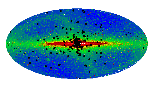
Globular clusters are gravitationally bound associations of 104 – 106 stars, distinct both from their smaller cousins, open clusters, and the larger, dark matter dominated dwarf galaxies that populate the low-mass end of the cosmological web of structure. Globular clusters are normally associated with a host galaxy and most galaxies, including the Milky Way, are surrounded and penetrated by a globular cluster system. A good estimate of the number of globular clusters in the Milky Way is the frequently updated catalogue by Harris [193 ], which has 157 entries as of 2010. Although fairly complete, a few new clusters
have been discovered in recent years at low Galactic latitudes [234, 271] and there may be
more hidden behind the galactic disc and bulge. The distribution of known globular clusters
in the Galaxy is given in Figure 1
], which has 157 entries as of 2010. Although fairly complete, a few new clusters
have been discovered in recent years at low Galactic latitudes [234, 271] and there may be
more hidden behind the galactic disc and bulge. The distribution of known globular clusters
in the Galaxy is given in Figure 1 . Other galaxies contain many more globular clusters and
the giant elliptical M87 alone may have over 10 000 [194]. The richness of the globular cluster
system of a galaxy can be classified by the number of globular clusters associated with the
galaxy normalized to its luminosity. One widely used measure of this is the specific frequency,
. Other galaxies contain many more globular clusters and
the giant elliptical M87 alone may have over 10 000 [194]. The richness of the globular cluster
system of a galaxy can be classified by the number of globular clusters associated with the
galaxy normalized to its luminosity. One widely used measure of this is the specific frequency,
 where
where  is the number of globular clusters and
  is the
 -band magnitude of the galaxy [195].
  can vary significantly between different galaxy
types. For instance
can vary significantly between different galaxy
types. For instance  for the local spiral galaxy M31 while
  for M87.
On the whole
for M87.
On the whole  seems to be higher in massive elliptical galaxies than in spiral galaxies.
For more information on extragalactic globular cluster systems see the review by Brodie &
Strader [61].
seems to be higher in massive elliptical galaxies than in spiral galaxies.
For more information on extragalactic globular cluster systems see the review by Brodie &
Strader [61].
Milky way globular clusters are old, having typical ages of 13 Gyr and an age spread of less than 5 Gyr [67]. This is on the order of the age of the Galaxy itself, thus Galactic globular clusters are thought to be left over from its formation. By contrast other galaxies such as the small and large Magellanic clouds (SMC and LMC) have intermediate age globular clusters (< 3 Gyr old, e.g., [346, 337]) and in some galaxy mergers, such as the Antennae, massive star-forming regions that may become globular clusters are observed [117]. Taken together, this implies that globular clusters of all ages are relatively common objects in the universe.
2.1 Stellar populations in globular clusters
Most of the detailed information on stellar populations in globular clusters comes from those in the Milky
Way since only they are close enough for stars to be individually resolved. The stars in individual Galactic
globular clusters all tend to have the same iron content [174] so globular clusters are thought to be
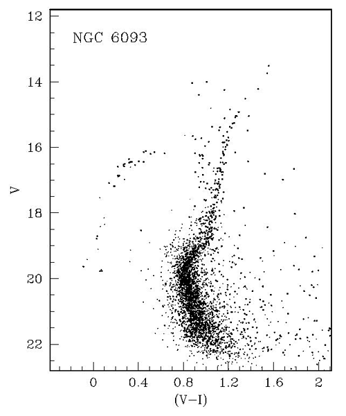
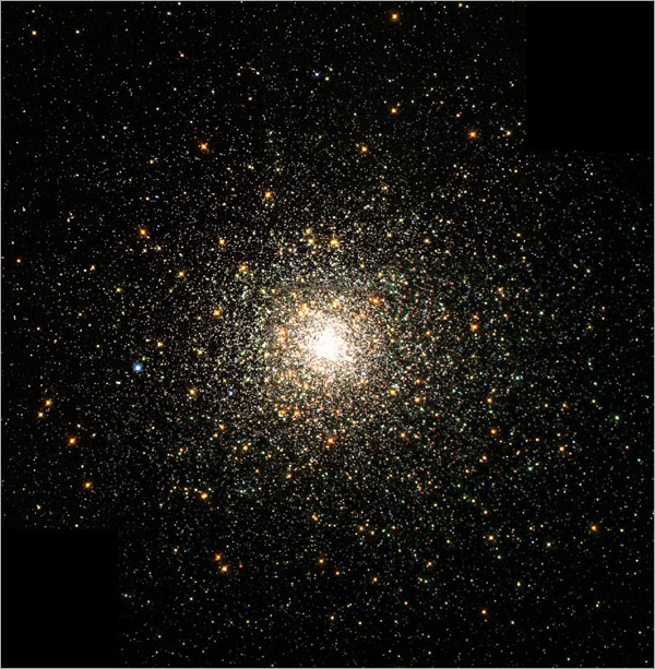
internally chemically homogeneous. The colour-magnitude diagram (CMDs) for most Galactic globular
clusters (e.g., M80, Figure 2) also indicate a single stellar population with a distinct main-sequence,
main-sequence turn-off, horizontal and giant branch. The single main sequence turn-off in particular
indicates that all stars in the cluster have the same age. This leads to a so-called “simple stellar population”
model for globular clusters where all stars have the same composition and age and differ only by
their masses, which are set by the initial mass function (IMF). This simple picture has been
challenged in recent years as observations have shown systematic star-to-star light element
variations in globular clusters [174, 376]. Specific effects include different populations in s-process
abundances (e.g., [321, 338]), anti-correlations between Na and O (e.g., [320, 321]), variations in
CNO elements (e.g., [321, 338]) and even differences in iron abundance (e.g., [320, 321]). The
best way of explaining these anomalies so far has been to use self-enrichment models where a
single globular cluster experiences several bursts of star formation, each enriched by pollution
from the previous generation [81]. How multiple populations affect the CMD of a globular
cluster is shown in Figure 3. The importance of these scenarios for relativistic binaries has
not yet been explored but if the first and second generation have different IMFs this could
affect the number of compact remnants. For this review, we will focus mainly on the case of a
simple stellar population but we will discuss details of the multi-generation case further in
Section 2.3.
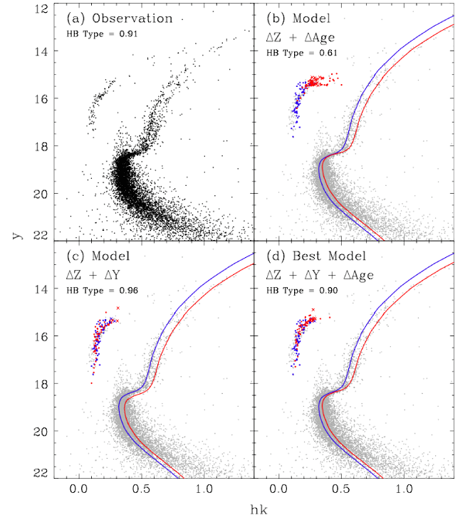
 Age = 1.5 Gyr. Image reproduced by permission from Roh et al. [412], copyright by IOP.
The IMF is thought to be universal [34] and is usually taken to be a power-law of the form
where
 is the mass of a star,
  the number of stars,
  is the number of stars in an
infinitesimal mass range and
is the number of stars in an
infinitesimal mass range and  can take different values for different mass ranges. For values above
 ,
,  is usually assumed to have a single value, the so-called Salpeter slope, of
  2.35 [416].
There is much more debate about the value of
2.35 [416].
There is much more debate about the value of  in low-mass regime. One solution is to treat the IMF as
a broken power-law with a break around
in low-mass regime. One solution is to treat the IMF as
a broken power-law with a break around  , such as that proposed by Kroupa & Weidner [279, 280]:
Another possibility, introduced by Chabrier [70], uses a log-normal distribution of masses below
, such as that proposed by Kroupa & Weidner [279, 280]:
Another possibility, introduced by Chabrier [70], uses a log-normal distribution of masses below 
 and a Salpeter slope above. In both cases the power-law strongly favours low masses so stars massive
enough to form neutron stars (NSs) and black holes (BHs) will be rare. It is worth noting that both of these
IMFs were derived in the context of clustered star formation and young open clusters in the solar
neighbourhood. It is often assumed that these IMFs hold for globular clusters as well but, because nearby
globular clusters are old, most of the stars above
and a Salpeter slope above. In both cases the power-law strongly favours low masses so stars massive
enough to form neutron stars (NSs) and black holes (BHs) will be rare. It is worth noting that both of these
IMFs were derived in the context of clustered star formation and young open clusters in the solar
neighbourhood. It is often assumed that these IMFs hold for globular clusters as well but, because nearby
globular clusters are old, most of the stars above  have already moved off the main-sequence.
Those just above
have already moved off the main-sequence.
Those just above  will be on the red giant branch and are readily visible in most optical
images of globular clusters, such as the image of M80 shown in Figure 4. Those that are more
massive have evolved past the giant and horizontal branches and become low-luminosity compact
remnants. The fact that the original high-mass population is no longer visible produces an intrinsic
uncertainty in our knowledge of the high-mass end of the IMF of globular cluster stars. It is
possible that the characteristic mass for star formation is higher in dense, optically thick regions
and this would lead to an IMF more biased towards high-mass stars [348]. This in turn would
increase the number of massive stellar remnants and could have an effect on the compact binary
population.
will be on the red giant branch and are readily visible in most optical
images of globular clusters, such as the image of M80 shown in Figure 4. Those that are more
massive have evolved past the giant and horizontal branches and become low-luminosity compact
remnants. The fact that the original high-mass population is no longer visible produces an intrinsic
uncertainty in our knowledge of the high-mass end of the IMF of globular cluster stars. It is
possible that the characteristic mass for star formation is higher in dense, optically thick regions
and this would lead to an IMF more biased towards high-mass stars [348]. This in turn would
increase the number of massive stellar remnants and could have an effect on the compact binary
population.
If we assume that the consequences of multiple stellar generations in globular clusers are negligible, then the picture of Galactic globular cluster stellar populations that emerges from this analysis is of a simple, nearly co-eval, chemically homogeneous set of luminous, low-mass population II stars combined with a low-luminosity population of high-mass stellar remnants. It is interactions with members of this remnant population that will be of particular interest for producing relativistic binaries.
2.2 The structure of globular clusters
Globular clusters are classically modelled as spherical N-body systems. This approximation is relatively
good given that the mean ellipticity,  , of Galactic globular clusters is
  (where
  ,
,
 is the semi-major axis and
  is the semi-minor axis) and that
  for all Galactic globular
clusters [193]. Globular clusters have a core-halo structure where the core is highly concentrated, reaching
densities of up to
for all Galactic globular
clusters [193]. Globular clusters have a core-halo structure where the core is highly concentrated, reaching
densities of up to  , and strongly self-gravitating. The surrounding halo is of much lower
density and is less strongly self-gravitating. The structure of a globular cluster can be classified using three
basic radii: the core radius (
, and strongly self-gravitating. The surrounding halo is of much lower
density and is less strongly self-gravitating. The structure of a globular cluster can be classified using three
basic radii: the core radius ( ), the half-mass radius (
 ), and the tidal radius (
 ). One
definition of the core radius relates it to the central velocity and density through the equation
). One
definition of the core radius relates it to the central velocity and density through the equation

 is the mean-squared central velocity and
  is the central density [199]. For an isothermal
model this corresponds roughly to the radius at which the density drops to about one third, and thus the
surface density to one half, of its central value. Observationally this corresponds to the radius at which the
surface brightness drops to half of its central value. For multi-mass systems it is less clear how to
arrive at an appropriate theoretical definition of the core radius and more empirical measures,
such as the density-weighted average of the distance of each star from the density center are
often used [68]. The half-mass radius is simply the radius thatcontains half of the mass of the
system. The corresponding observational value is the half-light radius, which contains half the
light of the system (the two radii do not necessarily agree). The tidal radius is the radius at
which the gravitational field of the host galaxy becomes more important than the self gravity of
the star cluster. A classical estimate of this for a circular orbit is given by Spitzer [443] as:
where
is the central density [199]. For an isothermal
model this corresponds roughly to the radius at which the density drops to about one third, and thus the
surface density to one half, of its central value. Observationally this corresponds to the radius at which the
surface brightness drops to half of its central value. For multi-mass systems it is less clear how to
arrive at an appropriate theoretical definition of the core radius and more empirical measures,
such as the density-weighted average of the distance of each star from the density center are
often used [68]. The half-mass radius is simply the radius thatcontains half of the mass of the
system. The corresponding observational value is the half-light radius, which contains half the
light of the system (the two radii do not necessarily agree). The tidal radius is the radius at
which the gravitational field of the host galaxy becomes more important than the self gravity of
the star cluster. A classical estimate of this for a circular orbit is given by Spitzer [443] as:
where 
 is the mass of the globular cluster,
  the mass of the galaxy and
  the
galactocentric radius of the circular orbit. In a time-dependent galactic field the escape process
becomes significantly more complicated (see [119] for a more complete theory of tidal escape in a
time-varyingexternal potential). For a given cluster, cluster orbit, and galaxy model the tidal radius of the
cluster can, in principle, be clearly defined by comparing the effect of the galactic versus globular cluster
gravitational field on a test mass. Observationally tidal radii can be difficult to determine due to the low
stellar density of globular cluster halos and an imperfect knowledge of the gravitational potential of the host
galaxy. Median values for
the
galactocentric radius of the circular orbit. In a time-dependent galactic field the escape process
becomes significantly more complicated (see [119] for a more complete theory of tidal escape in a
time-varyingexternal potential). For a given cluster, cluster orbit, and galaxy model the tidal radius of the
cluster can, in principle, be clearly defined by comparing the effect of the galactic versus globular cluster
gravitational field on a test mass. Observationally tidal radii can be difficult to determine due to the low
stellar density of globular cluster halos and an imperfect knowledge of the gravitational potential of the host
galaxy. Median values for  ,
,  , and
, and  in the Galaxy are
  1 pc,
1 pc,  3 pc and
  35 pc
respectively [199].
35 pc
respectively [199].
There are also two important timescales that characterize globular cluster evolution: the
crossing time ( ) and the relaxation time (
 ). The crossing time is simply the time
required for a star traveling at a typical velocity to cross some characteristic cluster radius. Thus,
). The crossing time is simply the time
required for a star traveling at a typical velocity to cross some characteristic cluster radius. Thus,
 where, for example,
  or
or  might be typical radii of interest and
  could be the
velocity dispersion – normally taken to be the root-mean-square velocity and observed to be
could be the
velocity dispersion – normally taken to be the root-mean-square velocity and observed to be
 10 km s–1 in Galactic globular clusters [193, 199].
  is also, roughly speaking, the
orbital timescale for the cluster. For typical values of
is also, roughly speaking, the
orbital timescale for the cluster. For typical values of  and
and  ,
,  for Galactic globular
clusters is on the order of 0.1 – 1 Myr but is longer at the tidal radius and much shorter in the
core.
for Galactic globular
clusters is on the order of 0.1 – 1 Myr but is longer at the tidal radius and much shorter in the
core.
The relaxation time describes how long it takes for orbits to be significantly altered by stellar
encounters. In particular  is often defined as the time necessary for the velocity of a star to change by
an order of itself [57]. This can be thought of as the time necessary for a cluster to lose the memory of its
initial conditions or, more exactly, the time necessary for stellar encounters to transform an
arbitrary velocity distribution to a Maxwellian [443]. The relaxation time is related to the number
and strength of encounters and, thus, to the number density and energy of a typical star in
the cluster. It can be shown that the mean relaxation time in a globular cluster is [57, 443]
is often defined as the time necessary for the velocity of a star to change by
an order of itself [57]. This can be thought of as the time necessary for a cluster to lose the memory of its
initial conditions or, more exactly, the time necessary for stellar encounters to transform an
arbitrary velocity distribution to a Maxwellian [443]. The relaxation time is related to the number
and strength of encounters and, thus, to the number density and energy of a typical star in
the cluster. It can be shown that the mean relaxation time in a globular cluster is [57, 443]

 and
and  as before, typical values of
  are 0.1 – 1 Gyr. Thus, with
ages typically greater than 10 Gyr, Galactic globular clusters are expected to be dynamically relaxed
objects. In reality the value of
are 0.1 – 1 Gyr. Thus, with
ages typically greater than 10 Gyr, Galactic globular clusters are expected to be dynamically relaxed
objects. In reality the value of  varies significantly within a globular cluster due to the highly
inhomogeneous density distribution of the core-halo structure. It is possible for the core of a globular cluster
to be fully relaxed while the halo remains un-relaxed after 13 Gyr. By making various approximations for
varies significantly within a globular cluster due to the highly
inhomogeneous density distribution of the core-halo structure. It is possible for the core of a globular cluster
to be fully relaxed while the halo remains un-relaxed after 13 Gyr. By making various approximations for
 it is possible to relate
  to local cluster properties. For instance the criterion of Meylan and
Heggie [326, 288]:
relates
to local cluster properties. For instance the criterion of Meylan and
Heggie [326, 288]:
relates 
 to the local mass density (
 ), the mass-weighted mean squared velocity (
 ), and the
average mass (
), and the
average mass ( ). The criterion by Spitzer [443]:
relates
). The criterion by Spitzer [443]:
relates 
 to a characteristic radius (
 ), the average mass, and the number of stars in the system. In
practise
), the average mass, and the number of stars in the system. In
practise  is normally used for the characteristic radius in the Spitzer criterion and
  is renamed the
half-mass relaxation time,
is renamed the
half-mass relaxation time,  . The factor
  that appears in both definitions is called the
Coulomb logarithm and describes the relative effectiveness of small and large angle collisions. It is
calculated as an integral over the impact parameters for two-body scattering encounters,
that appears in both definitions is called the
Coulomb logarithm and describes the relative effectiveness of small and large angle collisions. It is
calculated as an integral over the impact parameters for two-body scattering encounters,  :
where
:
where 
 is a constant of order unity. The exact value of
  is a matter of some debate and must be
determined empirically. Values in the literature range from 0.02 – 0.4 depending on the mass
distribution of the system [156, 157]. Both definitions of
is a matter of some debate and must be
determined empirically. Values in the literature range from 0.02 – 0.4 depending on the mass
distribution of the system [156, 157]. Both definitions of  are used extensively in stellar
dynamics.
are used extensively in stellar
dynamics.
On timescales shorter than a relaxation time interactions between individual stars do not govern the
overall evolution of a stellar system and the granularity of the gravitational potential can be ignored. On
these timescales the background structure of the cluster can be modelled using a static distribution
function,  , that describes the probability of finding a star at a particular location in a 6-D
position-velocity phase space. Formally,
, that describes the probability of finding a star at a particular location in a 6-D
position-velocity phase space. Formally,  depends on position, velocity, mass, and time so we have
 . For times less than
  , however, the evolution of
  is described by the collisionless
Boltzmann equation:
is described by the collisionless
Boltzmann equation:

 . The gravitational potential,
  , is given
by Poisson’s equation:
and can be calculated at any position by integrating the distribution function over mass and velocity:
Solutions to Eq. 9
, is given
by Poisson’s equation:
and can be calculated at any position by integrating the distribution function over mass and velocity:
Solutions to Eq. 9

 are often described in terms of the relative energy per unit mass,
  , rather
than in terms of the phase-space variables. Here,
, rather
than in terms of the phase-space variables. Here,  is the relative potential and
  is defined
such that no star has an energy less that zero (
is defined
such that no star has an energy less that zero ( for
for  and
and  for
for  ). A simple
class of solutions to Eq. 9 are Plummer models [378]:
the stellar-dynamical equivalent of an
). A simple
class of solutions to Eq. 9 are Plummer models [378]:
the stellar-dynamical equivalent of an 
 ploytrope [199]. Another class of models that admit
anisotropy and a distribution in angular momentum,
ploytrope [199]. Another class of models that admit
anisotropy and a distribution in angular momentum,  , are known as King–Mitchie models [264, 327].
Their basic distribution function is:
where
, are known as King–Mitchie models [264, 327].
Their basic distribution function is:
where ![2 [ ] f (ℰ,L) = ρ (2π σ2)−3∕2exp( −-L--) e ℰ∕σ2 − 1 , ℰ > 0 , (13 ) 1 2r2aσ2](article106x.gif)
 is the velocity dispersion,
  the anisotropy radius where the velocity distribution changes from
nearly isotropic to nearly radial, and
the anisotropy radius where the velocity distribution changes from
nearly isotropic to nearly radial, and  is a constant related to the density. Although not as well
theoretically supported as the single-mass case, King–Mitchie models have been extended to include a
spectrum of stellar masses [187] and even external gravitational field [200]. Multi-mass King models in
particular are often fit to observed globular cluster cluster surface brightness profiles in order to determine
their masses. A good example of the construction of a multi-mass King–Mitchie model is found in the
appendix of Miocchi [339].
is a constant related to the density. Although not as well
theoretically supported as the single-mass case, King–Mitchie models have been extended to include a
spectrum of stellar masses [187] and even external gravitational field [200]. Multi-mass King models in
particular are often fit to observed globular cluster cluster surface brightness profiles in order to determine
their masses. A good example of the construction of a multi-mass King–Mitchie model is found in the
appendix of Miocchi [339].
2.3 The dynamical evolution of globular clusters
Although static models can be used to describe the instantaneous structure of a globular cluster, there is no
stable equilibrium for self-gravitating systems [57] and, therefore, their structure changes dramatically over
time. Accessible descriptions of globular cluster evolution are given in Hut et al. [241], Meylan and
Heggie [326] and Meylan [325] and have also been the subject of several texts (e.g., Spitzer [443] and
Heggie and Hut [199]). Here we merely outline some of the more important aspects of globular cluster
evolution.
The initial conditions of globular clusters are not well constrained since they seem to form only very
early in the history of galaxy formation or in major mergers [150, 61] – both situations quite different from
the environment of our Galaxy today. However, it is possible to make some general statements. Like all
stars, the stars in globular clusters collapse out of molecular gas. Due to their small age spread and chemical
homogeneity, it seems likely that all the stars in a globular cluster formed by the collapse and fragmentation
of a single giant molecular cloud [61]. However, the exact details of how this collapse proceeds are unclear.
In the classical picture a globular cluster forms in a single collapse event – all stars form rapidly at almost
exactly the same time from a globally collapsing cloud of gas and, thus, have almost exactly the
same age and chemical composition. Not all of the gas in the collapsing cloud is necessarily
converted into stars and the fraction of gas that becomes stars is described through the star
formation efficiency (SFE). An SFE of less than 100% implies that not all of the primordial
gas forms stars and the resulting globular cluster will be less massive than its parent cloud.
Star formation is then terminated and the left-over gas expelled by a combination of ionizing
radiation from young stars and energy injection from supernovae. Although more applicable
to open clusters, Dale et al. [85] provides some the the most recent results on the details of
how this process works in young star clusters. If the star formation efficiency is low, then the
amount of mass loss through gas expulsion can leave the cluster out of virial equilibrium and may
lead to its immediate dissolution [171, 172, 484], a process called “infant mortality”. It is
estimated that more than half of young star clusters in the local universe are destroyed in this
manner [172] and even the surviving clusters will lose a large fraction of their stars. Even if
the cluster survives the gas expulsion, the rapid change in potential will cause the energy of
individual stars to change in a mass-independent manner [57]. This process, called violent
relaxation, means that the positions, velocities, and masses of cluster stars will be initially
uncorrelated.
As mentioned in Section 2.1, observations are now beginning to challenge some of the details of this
simplistic picture of globular cluster formation. Rather than a single burst of star formation the observed
abundance anomalies suggest a more drawn-out formation scenario where a first generation of
stars forms, evolves and enrichs the cloud with ejecta processed through nuclear burning. Later
generations form from the enriched gas and carry the chemical tracers of the pollution. A general
description of how such a scenario might proceed can be found in Conroy and Spergel [81] however
there is little consensus on the exact details. The initial cloud could suffer a global collapse,
experience star formation, have the collapse halted by feedback and then re-collapse to form the
second generation. Conversely, different regions of the cloud could collapse into sub-clumps at
different times and enrich neighbouring regions with their ejecta. The globular cluster would
then assemble from the merger of these sub-clumps. It is not clear what effect, if any, these
different formation scenarios will have on the compact binary population of globular clusters.
There is some suggestion that the early generations must have an IMF biased towards massive
stars in order to explain the observed abundance anomalies (e.g., [91, 92]) and if so this would
certainly have implications for the number of compact objects and compact binaries. However,
the question is far from resolved. Due to the uncertainties in the multi-generation scenarios
and in particular the fact that the details are not necessarily important for compact binary
production, we will assume a single star formation event in globular clusters for the purposes of this
review.
Equipartition of energy dictates that the most massive stars should have the lowest kinetic
energies [57, 443] but violent relaxation leaves the velocities and masses uncorrelated. Therefore, as soon as
the residual gas is expelled from a young globular cluster, massive stars with large kinetic energies will start
to transfer this energy to low-mass stars through stellar encounters. As the massive stars lose kinetic
energy they will sink to the center of the cluster while the low-mass stars gain kinetic energy
and move to the halo. This process is known as mass segregation and proceeds on a timescale
 [442, 479, 257]. Mass segregation can also occur in other situations, such as around
super-massive black holes in galactic centres [136]. Due to mass-loss from stellar evolution, compact
remnants rapidly become the most massive objects in globular clusters as the star population ages [419].
Thus they, along with binaries, are strongly affected by mass segregation and are particularly likely to be
found in cluster cores [475]. Mass segregation continues until energy equipartition has been
achieved. There are, however, initial conditions for which it is impossible to achieve energy
equipartition [479, 257] and it is formally impossible to halt mass segregation, leading to a
singularity in the core of the cluster. This phenomenon was first noted by Spitzer [442] and is thus
called the “Spitzer instability”. In reality, the massive objects in such systems form a strongly
interacting subsystem, dynamically decoupled from the rest of the cluster. Due to their high
masses, black holes in star clusters are particularly likely to experience the Spitzer instability
and this has been the starting point for several investigations of BH binaries in star clusters
(e.g. [360]).
[442, 479, 257]. Mass segregation can also occur in other situations, such as around
super-massive black holes in galactic centres [136]. Due to mass-loss from stellar evolution, compact
remnants rapidly become the most massive objects in globular clusters as the star population ages [419].
Thus they, along with binaries, are strongly affected by mass segregation and are particularly likely to be
found in cluster cores [475]. Mass segregation continues until energy equipartition has been
achieved. There are, however, initial conditions for which it is impossible to achieve energy
equipartition [479, 257] and it is formally impossible to halt mass segregation, leading to a
singularity in the core of the cluster. This phenomenon was first noted by Spitzer [442] and is thus
called the “Spitzer instability”. In reality, the massive objects in such systems form a strongly
interacting subsystem, dynamically decoupled from the rest of the cluster. Due to their high
masses, black holes in star clusters are particularly likely to experience the Spitzer instability
and this has been the starting point for several investigations of BH binaries in star clusters
(e.g. [360]).
The longer-term evolution of star clusters is driven by two-body relaxation, where the orbits of stars are
perturbed by encounters with their neighbours. The theory of two-body relaxation was first quantified by
Chandrasekhar in 1942 [71]. Two-body relaxation becomes important on timescales longer than the local
relaxation time. The evolution of a globular cluster over these timescales can still be described (at least
formally) by the Boltzmann equation but with a collisional term added to the right-hand side. Eq. 9 then
takes on the form:
![∂f- ⃗ ⃗ ∂f- ∂t + ⃗v ⋅ ∇f − ∇ϕ ⋅ ∂⃗v = Γ [f]. (14 )](article111x.gif) is sometimes called the collisional Boltzmann equation and the term
is sometimes called the collisional Boltzmann equation and the term ![Γ [f ]](article112x.gif) describes the effect of
two-body (and in principle higher-order) interactions on the distribution function. Practically speaking, it is
not possible to evaluate
describes the effect of
two-body (and in principle higher-order) interactions on the distribution function. Practically speaking, it is
not possible to evaluate ![Γ [f]](article113x.gif) analytically and various numerical approximations must be employed.
Approaches include the Fokker–Planck method, where
analytically and various numerical approximations must be employed.
Approaches include the Fokker–Planck method, where ![Γ [f]](article114x.gif) is approximated in the weak scattering limit
by an expansion in powers of the phase-space parameters; the Monte Carlo method, where
is approximated in the weak scattering limit
by an expansion in powers of the phase-space parameters; the Monte Carlo method, where ![Γ [f]](article115x.gif) is
approximated by a Monte Carlo selection of weak encounters over a time shorter than the relaxation time;
the anisotropic gas model where the cluster is approximated as a self-gravitating gaseous sphere; or direct
N-body integration, where rather than solving Eq. 14 the orbits of each star in the cluster are explicitly
integrated. Each method has its strengths and weaknesses and will be discussed further in
Section 5.
is
approximated by a Monte Carlo selection of weak encounters over a time shorter than the relaxation time;
the anisotropic gas model where the cluster is approximated as a self-gravitating gaseous sphere; or direct
N-body integration, where rather than solving Eq. 14 the orbits of each star in the cluster are explicitly
integrated. Each method has its strengths and weaknesses and will be discussed further in
Section 5.
Thermodynamically speaking, strongly self-gravitating systems have a negative heat capacity.
This can be seen by relating the kinetic energy of the system to a dynamical temperature [57]:


 are positive,
  is always negative. A negative
heat capacity means that heating a self-gravitating system actually causes it to lose energy. For a
core-halo star cluster, the core is strongly self-gravitating while the halo is not, so the halo
acts as a heat bath for the core. Any perturbation in which the core becomes dynamically
hotter than the halo causes energy to flow into the halo. The negative heat capacity means that
the core becomes even hotter, increasing the flow of energy to the halo in a runaway process.
This causes the core to contract, formally to a singularity. The runaway process is called the
gravothermal catastrophe and the consequent shrinking of the core is called core collapse. It affects all
self-gravitating systems and was first noted in the context of star clusters by Antonov [18]. In
equal-mass systems core collapse will occur after
is always negative. A negative
heat capacity means that heating a self-gravitating system actually causes it to lose energy. For a
core-halo star cluster, the core is strongly self-gravitating while the halo is not, so the halo
acts as a heat bath for the core. Any perturbation in which the core becomes dynamically
hotter than the halo causes energy to flow into the halo. The negative heat capacity means that
the core becomes even hotter, increasing the flow of energy to the halo in a runaway process.
This causes the core to contract, formally to a singularity. The runaway process is called the
gravothermal catastrophe and the consequent shrinking of the core is called core collapse. It affects all
self-gravitating systems and was first noted in the context of star clusters by Antonov [18]. In
equal-mass systems core collapse will occur after  [443] but may be accelerated in
systems with a spectrum of masses due to mass segregation. Core collapse not only appears
in analytic models, but has also been found in a variety of numerical simulations such as the
model shown in Figure 5 [253]. Furthermore, the Harris catalogue lists several Galactic globular
clusters that from their surface brightness profiles are thought to have experienced a core collapse
event [193].
[443] but may be accelerated in
systems with a spectrum of masses due to mass segregation. Core collapse not only appears
in analytic models, but has also been found in a variety of numerical simulations such as the
model shown in Figure 5 [253]. Furthermore, the Harris catalogue lists several Galactic globular
clusters that from their surface brightness profiles are thought to have experienced a core collapse
event [193].
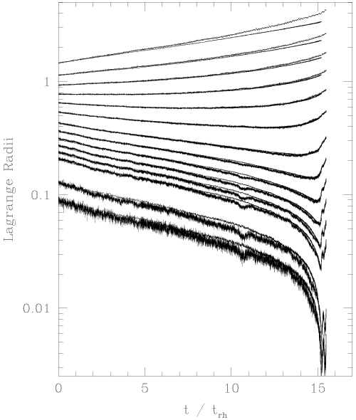 ], copyright by IOP.
 Core collapse can be halted, at least temporarily, by an energy source in the core. For stars (also
self-gravitating systems) this energy source is nuclear burning. In star clusters tightly bound binaries
perform a similar role. Stars in the core scatter off these binaries and gain kinetic energy at the expense of
the orbital energy of the binary. This process reverses the temperature gradient and consequently the
gravothermal instability which in turn causes the core to re-expand. The core will then cool again due to
the expansion, the temperature gradient will again reverse and the process of core collapse will repeat.
These repeated core expansions and contractions are know as gravothermal oscillations [56]. The heating
from the binaries is the trigger for the process and, in analogy to nuclear burning in stars, is
called “binary burning”. The binaries taking part in binary burning may be either primordial
(binaries where the stars were born bound to each other) or dynamically formed by a variety of
interactions that will be discussed in Section 4.3. It is worth noting that while tight binaries serve as
energy sources for the cluster, loosely bound binaries with orbital velocities below the local
velocity dispersion can actually act as energy sinks and may significantly hasten the onset of core
collapse [131]. The importance of this effect on the evolution of star clusters remains largely
unexplored.
Stars can escape from a star cluster if they gain a velocity greater than the cluster’s escape velocity,
 where
where  is the potential energy of the star cluster and
  its total mass. Using the
virial theorem it is possible to show that
its total mass. Using the
virial theorem it is possible to show that  where
where  is the RMS velocity in the
cluster [57]. There are two means through which a star can reach the escape velocity. The first is
ejection where a single strong interaction, such as occurs during binary burning, gives the star
a sufficient velocity impulse to exceed
is the RMS velocity in the
cluster [57]. There are two means through which a star can reach the escape velocity. The first is
ejection where a single strong interaction, such as occurs during binary burning, gives the star
a sufficient velocity impulse to exceed  . This process is highly stochastic. The second is
evaporation where a star reaches escape velocity due to a large number of weak encounters
during the relaxation process. Relaxation tends to maintain a local Maxwellian in the velocity
distribution and, since a Maxwellian distribution always has a fraction
. This process is highly stochastic. The second is
evaporation where a star reaches escape velocity due to a large number of weak encounters
during the relaxation process. Relaxation tends to maintain a local Maxwellian in the velocity
distribution and, since a Maxwellian distribution always has a fraction  stars with
 , there are always stars in the cluster with a velocity above the escape velocity.
Thus, it is the fate of all star clusters to evaporate. The evaporation time can be estimated as:
, there are always stars in the cluster with a velocity above the escape velocity.
Thus, it is the fate of all star clusters to evaporate. The evaporation time can be estimated as:

 are stripped from the cluster and lost. Tidal dynamics are more complicated than a
simple radial cutoff would imply and detailed prescriptions taking into account orbital energy and angular
momentum as well as a time-varying field for star clusters in elliptical orbits are necessary to capture all of
the important processes [457, 119]. It seems likely that the ultimate fate of most globular clusters is
destruction due to tidal effects [167, 152]. Since most compact objects are likely to live deep in the
core of globular clusters where ejection will normally be due to violent interactions, the details
of tidal stripping are unlikely to be critical for the treatment of relativistic binaries in star
clusters.
are stripped from the cluster and lost. Tidal dynamics are more complicated than a
simple radial cutoff would imply and detailed prescriptions taking into account orbital energy and angular
momentum as well as a time-varying field for star clusters in elliptical orbits are necessary to capture all of
the important processes [457, 119]. It seems likely that the ultimate fate of most globular clusters is
destruction due to tidal effects [167, 152]. Since most compact objects are likely to live deep in the
core of globular clusters where ejection will normally be due to violent interactions, the details
of tidal stripping are unlikely to be critical for the treatment of relativistic binaries in star
clusters.
 |
 |
 |
Living Rev. Relativity, 16 (2013), 4, doi:10.12942/lrr-2013-4, URL (accessed <date>): http://www.livingreviews.org/lrr-2013-4.
 This work is licensed under a Creative Commons License.
© The author(s), except where otherwise noted.
This work is licensed under a Creative Commons License.
© The author(s), except where otherwise noted.