6 Numerical Relativity
Generating time-dependent solutions to the Einstein equations using numerical methods involves an extended list of ingredients which can be loosely summarized as follows.- Cast the field equations as an IBVP.
- Choose a specific formulation that admits a well-posed IBVP, i.e., there exist suitable choices for the following ingredients that ensure well posedness.
- Choose numerically suitable coordinate or gauge conditions.
- Discretize the resulting set of equations.
- Handle singularities such that they do not result in the generation of non-assigned numbers which rapidly swamp the computational domain.
- Construct initial data that solve the Einstein constraint equations and represent a realistic snapshot of the physical system under consideration.
- Specify suitable outer boundary conditions.
- Fix technical aspects: mesh refinement and/or multi-domains as well as use of multiple computer processors through parallelization.
- Apply diagnostic tools that measure GWs, BH horizons, momenta and masses, and other fields.
In this section, we will discuss state-of-the-art choices for these ingredients.
6.1 Formulations of the Einstein equations
6.1.1 The ADM equations
The Einstein equations in dimensions describing a spacetime with
cosmological constant
dimensions describing a spacetime with
cosmological constant  and energy-matter content
  are given by
Elegant though this tensorial form of the equations is from a mathematical point of view, it is not
immediately suitable for a numerical implementation. For one thing, the character of the equations as a
hyperbolic, parabolic or elliptic system is not evident. In other words, are we dealing with an initial-value or
a boundary-value problem? In fact, the Einstein equations are of mixed character in this regard
and represent an IBVP. Well-posedness of the IBVP then requires a suitable formulation of
the evolution equations, boundary conditions and initial data. We shall discuss this particular
aspect in more detail further below, but first consider the general structure of the equations.
The multitude of possible ways of writing the Einstein equations are commonly referred to as
formulations of the equations and a good starting point for their discussion is the canonical “3 + 1” or
“
are given by
Elegant though this tensorial form of the equations is from a mathematical point of view, it is not
immediately suitable for a numerical implementation. For one thing, the character of the equations as a
hyperbolic, parabolic or elliptic system is not evident. In other words, are we dealing with an initial-value or
a boundary-value problem? In fact, the Einstein equations are of mixed character in this regard
and represent an IBVP. Well-posedness of the IBVP then requires a suitable formulation of
the evolution equations, boundary conditions and initial data. We shall discuss this particular
aspect in more detail further below, but first consider the general structure of the equations.
The multitude of possible ways of writing the Einstein equations are commonly referred to as
formulations of the equations and a good starting point for their discussion is the canonical “3 + 1” or
“
 ” split originally developed by Arnowitt, Deser & Misner [47*] and later reformulated by
York [810, 812].
” split originally developed by Arnowitt, Deser & Misner [47*] and later reformulated by
York [810, 812].
The tensorial form of the Einstein equations (39*) fully reflects the unified viewpoint of space and time; it is only through
the Lorentzian signature  of the metric that the timelike character of one of the coordinates manifests
itself.9
It turns out crucial for understanding the character of Einstein’s equations to make the distinction between
spacelike and timelike coordinates more explicit.
of the metric that the timelike character of one of the coordinates manifests
itself.9
It turns out crucial for understanding the character of Einstein’s equations to make the distinction between
spacelike and timelike coordinates more explicit.
Let us consider for this purpose a spacetime described by a manifold  equipped with a metric
  of Lorentzian signature. We shall further assume that there exists a foliation of the spacetime in the sense
that there exists a scalar function
of Lorentzian signature. We shall further assume that there exists a foliation of the spacetime in the sense
that there exists a scalar function  with the following properties. (i) The 1-form
  associated with the function
  is timelike everywhere; (ii) The hypersurfaces
  defined by
  are non-intersecting and
  . Points inside each hypersurface
  are labelled by spatial
coordinates
are labelled by spatial
coordinates  , and we refer to the coordinate system
  as adapted to the
spacetime split.
as adapted to the
spacetime split.
Next, we define the lapse function  and shift vector
  through

 is the timelike unit normal field. The geometrical interpretation of these quantities in
terms of the timelike unit normal field
is the timelike unit normal field. The geometrical interpretation of these quantities in
terms of the timelike unit normal field  and the coordinate basis vector
  is illustrated in
Figure 2*. Using the relation
is illustrated in
Figure 2*. Using the relation  and the definition of
  and
and  , one directly finds
 , so that the shift
  is tangent to the hypersurfaces
  . It measures the deviation
of the coordinate vector
. It measures the deviation
of the coordinate vector  from the normal direction
  . The lapse function relates the
proper time measured by an observer moving with four velocity
. The lapse function relates the
proper time measured by an observer moving with four velocity  to the coordinate time
  :
:
 .
.
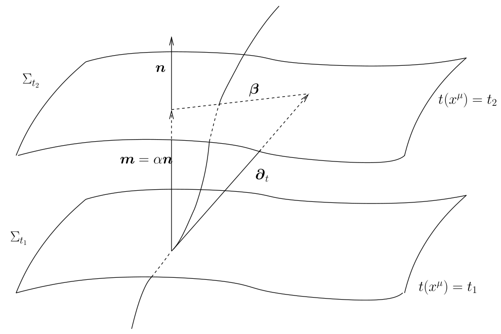
 . Lapse
  and shift
  are defined
by the relation of the timelike unit normal field
are defined
by the relation of the timelike unit normal field  and the basis vector
  associated with the
coordinate
associated with the
coordinate  . Note that
  and, hence, the shift vector
  is tangent to
  .
. A key ingredient for the spacetime split of the equations is the projection of tensors onto time and space
directions. For this purpose, the space projection operator is defined as  . For a
generic tensor
. For a
generic tensor  , its spatial projection is given by projecting each index speparately

 is called tangent to
  if it is invariant under projection, i.e.,
  . In adapted
coordinates, we can ignore the time components of such spatial tensors and it is common practice to denote
their components with Latin indices
. In adapted
coordinates, we can ignore the time components of such spatial tensors and it is common practice to denote
their components with Latin indices  . We similarly obtain time projections of a
tensor by contracting its indices with
. We similarly obtain time projections of a
tensor by contracting its indices with  . Mixed projections are obtained by contracting any
combination of tensor indices with
. Mixed projections are obtained by contracting any
combination of tensor indices with  and projecting the remaining ones with
  . A
particularly important tensor is obtained from the spatial projection of the spacetime metric
. A
particularly important tensor is obtained from the spatial projection of the spacetime metric

 is known as the first fundamental form or spatial metric and describes the intrinsic geometry of the
spatial hypersurfaces
is known as the first fundamental form or spatial metric and describes the intrinsic geometry of the
spatial hypersurfaces  . As we see from Eq. (42*), it is identical to the projection operator. In the
remainder, we will use both the
. As we see from Eq. (42*), it is identical to the projection operator. In the
remainder, we will use both the  and
and  symbols to denote this tensor depending on whether the
emphasis is on the projection or the hypersurface geometry.
symbols to denote this tensor depending on whether the
emphasis is on the projection or the hypersurface geometry.
With our definitions, it is straightforward to show that the spacetime metric in adapted coordinates
 can be written as
  or, equivalently,

 defines a unique, torsion-free and metric-compatible
connection
defines a unique, torsion-free and metric-compatible
connection  whose covariant derivative for an arbitrary spatial
tensor is given by
whose covariant derivative for an arbitrary spatial
tensor is given by

The final ingredient required for the spacetime split of the Einstein equations is the extrinsic curvature or second fundamental form defined as
The sign convention employed here is common in NR but the “
 ” is sometimes omitted in other
studies of GR. The definition (45*) provides an intuitive geometric interpretation of the extrinsic
curvature as the change in direction of the timelike unit normal field
” is sometimes omitted in other
studies of GR. The definition (45*) provides an intuitive geometric interpretation of the extrinsic
curvature as the change in direction of the timelike unit normal field  as we move across the
hypersurface
as we move across the
hypersurface  . As indicated by its name, the extrinsic curvature thus describes the embedding of
 inside the higher-dimensional spacetime manifold. The projection
  is symmetric
under exchange of its indices in contrast to its non-projected counterpart
is symmetric
under exchange of its indices in contrast to its non-projected counterpart  . For the
formulation of the Einstein equations in the spacetime split, it is helpful to introduce the vector field
. For the
formulation of the Einstein equations in the spacetime split, it is helpful to introduce the vector field
 . A straightforward calculation shows that the extrinsic curvature can be
expressed in terms of the Lie derivative of the spatial metric along either
. A straightforward calculation shows that the extrinsic curvature can be
expressed in terms of the Lie derivative of the spatial metric along either  or
or  according to

We have now assembled all tools to calculate the spacetime projections of the Riemann tensor. In the following order, these are known as the Gauss, the contracted Gauss, the scalar Gauss, the Codazzi, the contracted Codazzi equation, as well as the final projection of the Riemann tensor and its contractions:
Here,
 denotes the Riemann tensor and its contractions as defined in standard fashion from the spatial
metric
denotes the Riemann tensor and its contractions as defined in standard fashion from the spatial
metric  . For simplicity, we have kept all spacetime indices here even for spatial tensors. As mentioned
above, the time components can and will be discarded eventually.
. For simplicity, we have kept all spacetime indices here even for spatial tensors. As mentioned
above, the time components can and will be discarded eventually.
By using Eq. (47*), we can express the space and time projections of the Einstein equations (39*) exclusively in terms of the first and second fundamental forms and their derivatives. It turns out helpful for this purpose to introduce the corresponding projections of the energy-momentum tensor which are given by
Then, the energy-momentum tensor is reconstructed according to
 .
Using the explicit expressions for the Lie derivatives
we obtain the spacetime split of the Einstein equations
By virtue of the Bianchi identities, the constraints (54*) and (55*) are preserved under the evolution
equations. Furthermore, we can see that
.
Using the explicit expressions for the Lie derivatives
we obtain the spacetime split of the Einstein equations
By virtue of the Bianchi identities, the constraints (54*) and (55*) are preserved under the evolution
equations. Furthermore, we can see that 
 second-order-in-time evolution equations for the
 are written as a first-order-in-time system through introduction of the extrinsic curvature.
Additionally, we have obtained
are written as a first-order-in-time system through introduction of the extrinsic curvature.
Additionally, we have obtained  constraint equations, the Hamiltonian and momentum constraints,
which relate data within a hypersurface
constraint equations, the Hamiltonian and momentum constraints,
which relate data within a hypersurface  . We note that the Einstein equations do not determine the
lapse
. We note that the Einstein equations do not determine the
lapse  and shift
  . For the case of
  , these equations are often referred to as the ADM
equations, although we note that Arnowitt, Deser & Misner used the canonical momentum in place of the
extrinsic curvature in their original work [47*]. Counting the degrees of freedom, we start with
, these equations are often referred to as the ADM
equations, although we note that Arnowitt, Deser & Misner used the canonical momentum in place of the
extrinsic curvature in their original work [47*]. Counting the degrees of freedom, we start with
 components of the spacetime metric. The Hamiltonian and momentum constraints determine
 of these while
  gauge functions represent the gauge freedom, leaving
  physical
degrees of freedom as expected.
physical
degrees of freedom as expected.
6.1.2 Well-posedness
The suitability of a given system of differential equations for a numerical time evolution critically depends on a continuous dependency of the solution on the initial data. This aspect is referred to as well posedness of the IBVP and is discussed in great detail in Living Reviews articles and other works [645*, 674*, 383, 427]. Here, we merely list the basic concepts and refer the interested reader to these articles.Consider for simplicity an initial-value problem in one space and one time dimension for a single variable
 on an unbounded domain. Well-posedness requires a norm
  , i.e., a map from the space of
functions
, i.e., a map from the space of
functions  to the real numbers
  , and a function
  independent of the initial data such that

 denotes a linear perturbation relative to a solution
  [380*]. We note that
  may
be a rapidly growing function, for example an exponential, so that well posedness represents a necessary but
not sufficient criterion for suitability of a numerical scheme.
may
be a rapidly growing function, for example an exponential, so that well posedness represents a necessary but
not sufficient criterion for suitability of a numerical scheme.
Well posedness of formulations of the Einstein equations is typically studied in terms of the
hyperbolicity properties of the system in question. Hyperbolicity of a system of PDEs is often defined
in terms of the principal part, that is, the terms of the PDE which contain the highest-order
derivatives. We consider for simplicity a quasilinear first-order system for a set of variables 

 is a smooth differential operator and its associated principal
symbol is symmetrizeable [567*]. For the special case of constant coefficient systems this definition simplifies
to the requirement that the principal symbol has only imaginary eigenvalues and a complete set of linearly
independent eigenvectors. If linear independence of the eigenvectors is not satisfied, the system is called
weakly hyperbolic. For more complex systems of equations, strong and weak hyperbolicity can be defined in
a more general fashion [645, 567*, 646, 674*].
is a smooth differential operator and its associated principal
symbol is symmetrizeable [567*]. For the special case of constant coefficient systems this definition simplifies
to the requirement that the principal symbol has only imaginary eigenvalues and a complete set of linearly
independent eigenvectors. If linear independence of the eigenvectors is not satisfied, the system is called
weakly hyperbolic. For more complex systems of equations, strong and weak hyperbolicity can be defined in
a more general fashion [645, 567*, 646, 674*].
In our context, it is of particular importance that strong hyperbolicity is a necessary condition for a well posed IBVP [741, 742]. The ADM equations (52*) – (53*), in contrast, have been shown to be weakly but not strongly hyperbolic for fixed gauge [567]; likewise, a first-order reduction of the ADM equations has been shown to be weakly hyperbolic [468]. These results strongly indicate that the ADM formulation is not suitable for numerical evolutions of generic spacetimes.
A modification of the ADM equations which has been used with great success in NR is the BSSN system [78, 695] which is the subject of the next section.
6.1.3 The BSSN equations
It is interesting to note that the BSSN formulation had been developed in the 1990s before a comprehensive understanding of the hyperbolicity properties of the Einstein equations had been obtained; it was only about a decade after its first numerical application that strong hyperbolicity of the BSSN system [380] was demonstrated. We see here an example of how powerful a largely empirical approach can be in the derivation of successful numerical methods. And yet, our understanding of the mathematical properties is of more than academic interest as we shall see in Section 6.1.5 below when we discuss recent investigations of potential improvements of the BSSN system.The modification of the ADM equations which results in the BSSN formulation consists of a trace split of
the extrinsic curvature, a conformal decomposition of the spatial metric and of the traceless
part of the extrinsic curvature and the introduction of the contracted Christoffel symbols as
independent variables. For generality, we will again write the definitions of the variables and
the equations for the case of an arbitrary number  of spacetime dimensions. We define
 and
and  is the Christoffel symbol defined in the usual manner in terms of the
conformal metric
is the Christoffel symbol defined in the usual manner in terms of the
conformal metric  . Note that the definition (58*) implies two algebraic and one differential constraints

Inserting the definition (58*) into the ADM equations (52*) – (53*) and using the Hamiltonian and
momentum constraints respectively in the evolution equations for  and
and  results in the BSSN
evolution system
results in the BSSN
evolution system
![M --2--- M ∂tχ = β ∂M χ + D − 1 χ(αK − ∂M β ), (60 ) 2 ∂t&tidle;γIJ = βM∂M &tidle;γIJ + 2&tidle;γM (I∂J)βM − ------&tidle;γIJ∂MβM − 2α &tidle;AIJ, (61 ) D − 1 M MN &tidle;MN &tidle; --1--- 2 ∂tK = β ∂M K − χγ&tidle; DM DN α + α A AMN + D − 1 αK 8π 2 + ------α[S + (D − 3 )ρ ] −------α Λ, (62 ) D − 2 D − 2 ∂ A&tidle; = βM∂ A&tidle; + 2A&tidle; ∂ βM − --2---&tidle;A ∂ βM + αK A&tidle; − 2α &tidle;A &tidle;AM t IJ M IJ M (I J) D − 1 IJ M IJ IM J +χ (αℛ − D D α − 8παS )TF , (63 ) IJ I J IJ ∂ &tidle;Γ I = βM∂ &tidle;Γ I +---2--&tidle;Γ I∂ βM − &tidle;Γ M ∂ βI + &tidle;γMN ∂ ∂ βI + D-−-3-&tidle;γIM∂ ∂ βN t M D − 1 M M M N D − 1 M N [ ∂M χ ] D − 2 α −A&tidle;IM (D − 1 )α -----+ 2∂M α + 2 α&tidle;Γ IMN &tidle;AMN − 2------α &tidle;γIM∂M K − 16π -jI. (64 ) χ D − 1 χ](article539x.gif)
![1 Γ IJK = &tidle;Γ IJK −--(δIK∂J χ + δIJ∂Kχ − &tidle;γJK &tidle;γIM∂M χ) , (65 ) 2χ ℛIJ = ℛ&tidle;IJ + ℛ χIJ, (66 ) [ ] ( ) ℛ χIJ = &tidle;γIJ &tidle;γMN D&tidle;M D&tidle;N χ − D-−--1&tidle;γMN ∂M χ∂N χ + D--−-3 D&tidle;I D&tidle;J χ − -1-∂Iχ ∂Jχ , (67 ) 2 χ 2χ 2χ 2 χ 1 MN M M MN [ K K ] ℛ&tidle;IJ = − -&tidle;γ ∂N ∂Nγ&tidle;IJ + &tidle;γM (I∂J)&tidle;Γ + Γ&tidle; &tidle;Γ(IJ)M + &tidle;γ 2&tidle;ΓM(I&tidle;ΓJ)KN + &tidle;ΓIM &tidle;ΓKJN , (68 ) 2 1 1 DIDJ α = D&tidle;I &tidle;DJ α + --∂(Iχ ∂J)α − ---&tidle;γIJγ&tidle;MN ∂Mχ ∂Nα. (69 ) χ 2χ](article540x.gif)
 whereas enforcement of the unit determinant
  appears to be optional. A further
subtlety is concerned with the presence of the conformal connection functions
appears to be optional. A further
subtlety is concerned with the presence of the conformal connection functions  on the right-hand side of
the BSSN equations. Two recipes have been identified that provide long-term stable numerical evolutions.
(i) The independently evolved
on the right-hand side of
the BSSN equations. Two recipes have been identified that provide long-term stable numerical evolutions.
(i) The independently evolved  are only used when they appear in differentiated form but are replaced
by their definition in terms of the conformal metric
are only used when they appear in differentiated form but are replaced
by their definition in terms of the conformal metric  everywhere else [23*]. (ii) Alternatively,
one can add to the right-hand side of Eq. (64*) a term
everywhere else [23*]. (ii) Alternatively,
one can add to the right-hand side of Eq. (64*) a term  , where
  is a positive
constant [803].
is a positive
constant [803].
We finally note that in place of the variable  , alternative choices for evolving the conformal factor are
in use in some NR codes, namely
, alternative choices for evolving the conformal factor are
in use in some NR codes, namely  [65*] or
  [540]. An overview of the specific
choices of variables and treatment of the BSSN constraints for the present generation of codes is given in
Section 4 of [429*].
[540]. An overview of the specific
choices of variables and treatment of the BSSN constraints for the present generation of codes is given in
Section 4 of [429*].
6.1.4 The generalized harmonic gauge formulation
It has been realized a long time ago that the Einstein equations have a mathematically appealing form if one imposes the harmonic gauge condition [294]. Taking the derivative of this condition eliminates a specific combination of
second derivatives from the Ricci tensor such that its principal part is that of the scalar wave operator
where the dots denote terms involving at most the first derivative of the metric. In consequence of this
simplification of the principal part, the Einstein equations in harmonic gauge can straightforwardly be
written as a strongly hyperbolic system. This formulation even satisfies the stronger condition of symmetric
hyperbolicity which is defined in terms of the existence of a conserved, positive energy [674], and harmonic
coordinates have played a key part in establishing local uniqueness of the solution to the Cauchy problem in
GR [327, 141, 321].
[294]. Taking the derivative of this condition eliminates a specific combination of
second derivatives from the Ricci tensor such that its principal part is that of the scalar wave operator
where the dots denote terms involving at most the first derivative of the metric. In consequence of this
simplification of the principal part, the Einstein equations in harmonic gauge can straightforwardly be
written as a strongly hyperbolic system. This formulation even satisfies the stronger condition of symmetric
hyperbolicity which is defined in terms of the existence of a conserved, positive energy [674], and harmonic
coordinates have played a key part in establishing local uniqueness of the solution to the Cauchy problem in
GR [327, 141, 321].

This particularly appealing property of the Ricci tensor can be maintained for arbitrary coordinates by introducing the functions [333, 343*]
and promoting them to the status of independently evolved variables; see also [630*, 519*]. This is called the Generalized Harmonic Gauge formulation.
With this definition, it turns out convenient to consider the generalized class of equations
where
 . The addition of the term
  replaces the contribution of
  to the
Ricci tensor in terms of
to the
Ricci tensor in terms of  and thus changes the principal part to that of the scalar wave operator. A
solution to the Einstein equations is now obtained by solving Eq. (72*) subject to the constraint
and thus changes the principal part to that of the scalar wave operator. A
solution to the Einstein equations is now obtained by solving Eq. (72*) subject to the constraint
 .
.
The starting point for a Cauchy evolution are initial data  and
and  which satisfy the
constraints
which satisfy the
constraints  . A convenient manner to construct such initial data is to compute the initial
 directly from Eq. (71*) so that
  by construction. It can then be shown [519*] that the ADM
constraints (54*), (55*) imply
by construction. It can then be shown [519*] that the ADM
constraints (54*), (55*) imply  . By virtue of the contracted Bianchi identities, the evolution of the
constraint system obeys the equation
. By virtue of the contracted Bianchi identities, the evolution of the
constraint system obeys the equation
![[ ( ) ] μ μ 1 2 □ 𝒞α = − 𝒞 ∇ (μ𝒞α) − 𝒞 8 π Tμα − D--−-2T gμα + D-−--2Λg μα , (73 )](article566x.gif)
 is preserved under time evolution in the continuum limit.
A key addition to the GHG formalism has been devised by Gundlach et al. [377*] in the form of
damping terms which prevent growth of numerical violations of the constraints  due to
discretization or roundoff errors.
due to
discretization or roundoff errors.
Including these damping terms and using the definition (71*) to substitute higher derivatives in the Ricci tensor, the generalized Einstein equations (72*) can be written as
where![μν μν μ μ ν g ∂μ∂ νgαβ = − 2 ∂νgμ(α ∂β)g − 2 ∂(αH β) + 2H μΓαβ − 2Γ ναΓμβ 8πT--−-2Λ- [ μ ] − 8 πTαβ + D − 2 gαβ − 2κ 2n(α𝒞β) − λgαβn 𝒞μ , (74 )](article569x.gif)
 ,
,  are user-specified constraint-damping parameters. An alternative first-order system of the
GHG formulation has been presented in Ref. [519].
are user-specified constraint-damping parameters. An alternative first-order system of the
GHG formulation has been presented in Ref. [519].
6.1.5 Beyond BSSN: Improvements for future applications
The vast majority of BH evolutions in generic -dimensional spacetimes have been performed with the GHG and the BSSN formulations. It is
interesting to note in this context the complementary nature of the two formulations’ respective strengths
and weaknesses. In particular, the constraint subsystem of the BSSN equations contains a zero-speed mode
[100, 379, 378] which may lead to large Hamiltonian constraint violations. The GHG system does not
contain such modes and furthermore admits a simple way of controlling constraint violations in the form of
damping terms [377]. Finally, the wave-equation-type principal part of the GHG system allows for the
straightforward construction of constraint-preserving boundary conditions [650, 492*, 665*]. On the other
hand, the BSSN formulation is remarkably robust and allows for the simulation of BH binaries over a wide
range of the parameter space with little if any modifications of the gauge conditions; cf. Section 6.4.
Combination of these advantages in a single system has motivated the exploration of improvements to the
BSSN system and in recent years resulted in the identification of a conformal version of the
-dimensional spacetimes have been performed with the GHG and the BSSN formulations. It is
interesting to note in this context the complementary nature of the two formulations’ respective strengths
and weaknesses. In particular, the constraint subsystem of the BSSN equations contains a zero-speed mode
[100, 379, 378] which may lead to large Hamiltonian constraint violations. The GHG system does not
contain such modes and furthermore admits a simple way of controlling constraint violations in the form of
damping terms [377]. Finally, the wave-equation-type principal part of the GHG system allows for the
straightforward construction of constraint-preserving boundary conditions [650, 492*, 665*]. On the other
hand, the BSSN formulation is remarkably robust and allows for the simulation of BH binaries over a wide
range of the parameter space with little if any modifications of the gauge conditions; cf. Section 6.4.
Combination of these advantages in a single system has motivated the exploration of improvements to the
BSSN system and in recent years resulted in the identification of a conformal version of the
 system, originally developed in Refs. [113, 112, 114], as a highly promising candidate
[28*, 163*, 775, 428*].
system, originally developed in Refs. [113, 112, 114], as a highly promising candidate
[28*, 163*, 775, 428*].
The key idea behind the  system is to replace the Einstein equations with a generalized class of
equations given by
system is to replace the Einstein equations with a generalized class of
equations given by
![G = 8πT − ∇ Z − ∇ Z + g ∇ Zμ + κ [n Z + n Z + κ g n ZM ], (75 ) αβ αβ α β β α αβ μ 1 α β β α 2 αβ M](article575x.gif)
 is a vector field of constraints which is decomposed into space and time components according
to
is a vector field of constraints which is decomposed into space and time components according
to  and
and  . Clearly, a solution to the Einstein equations is recovered provided the
constraint
. Clearly, a solution to the Einstein equations is recovered provided the
constraint  is satisfied. The conformal version of the
  system is obtained in the same manner
as for the BSSN system and leads to time evolution equations for a set of variables nearly identical to the
BSSN variables but augmented by the constraint variable
system is obtained in the same manner
as for the BSSN system and leads to time evolution equations for a set of variables nearly identical to the
BSSN variables but augmented by the constraint variable  . The resulting evolution equations given in
the literature vary in details, but clearly represent relatively minor modifications for existing BSSN codes
[28*, 163, 428*]. Investigations have shown that the conformal
. The resulting evolution equations given in
the literature vary in details, but clearly represent relatively minor modifications for existing BSSN codes
[28*, 163, 428*]. Investigations have shown that the conformal  system is indeed suitable for
implementation of constraint preserving boundary conditions [664] and that constraint violations in
simulations of gauge waves and BH and NS spacetimes are indeed smaller than those obtained for
the BSSN system, in particular when constraint damping is actively enforced [28, 428*]. This
behaviour also manifests itself in more accurate results for the gravitational radiation in binary
inspirals [428*]. In summary, the conformal
system is indeed suitable for
implementation of constraint preserving boundary conditions [664] and that constraint violations in
simulations of gauge waves and BH and NS spacetimes are indeed smaller than those obtained for
the BSSN system, in particular when constraint damping is actively enforced [28, 428*]. This
behaviour also manifests itself in more accurate results for the gravitational radiation in binary
inspirals [428*]. In summary, the conformal  formulation is a very promising candidate for
future numerical studies of BH spacetimes, including in particular the asymptotically AdS
case where a rigorous control of the outer boundary is of utmost importance; cf. Section 6.6
below.
formulation is a very promising candidate for
future numerical studies of BH spacetimes, including in particular the asymptotically AdS
case where a rigorous control of the outer boundary is of utmost importance; cf. Section 6.6
below.
Another modification of the BSSN equations is based on the use of densitized versions of the trace of the extrinsic curvature and the lapse function as well as the traceless part of the extrinsic curvature with mixed indices [497, 795]. Some improvements in simulations of colliding BHs in higher-dimensional spacetimes have been found by careful exploration of the densitization parameter space [791*].
6.1.6 Alternative formulations
The formulations discussed in the previous subsections are based on a spacetime split of the Einstein equations. A natural alternative to such a split is given by the characteristic approach pioneered by Bondi et al. and Sachs [118*, 667*]. Here, at least one coordinate is null and thus adapted to the characteristics of the vacuum Einstein equations. For generic four-dimensional spacetimes with no symmetry assumptions, the characteristic formalism results in a natural hierarchy of two evolution equations, four hypersurface equations relating variables on hypersurfaces of constant retarded (or advanced) time, as well as three supplementary and one trivial equations. A comprehensive overview of characteristic methods in NR is given in the Living Reviews article [788*]. Although characteristic codes have been developed with great success in spacetimes with additional symmetry assumptions, evolutions of generic BH spacetimes face the problem of formation of caustics, resulting in a breakdown of the coordinate system; see [59] for a recent investigation. One possibility to avoid the problem of caustic formation is Cauchy-characteristic matching, the combination of a or Cauchy-type numerical scheme in the interior strong-field region with a characteristic
scheme in the outer parts. In the form of Cauchy-characteristic extraction, i.e., ignoring the
injection of information from the characteristic evolution into the inner Cauchy region, this
approach has been used to extract GWs with high accuracy from numerical simulations of compact
objects [642*, 60*].
or Cauchy-type numerical scheme in the interior strong-field region with a characteristic
scheme in the outer parts. In the form of Cauchy-characteristic extraction, i.e., ignoring the
injection of information from the characteristic evolution into the inner Cauchy region, this
approach has been used to extract GWs with high accuracy from numerical simulations of compact
objects [642*, 60*].
All the Cauchy and characteristic or combined approaches we have discussed so far, evolve the physical
spacetime, i.e., a manifold with metric  . An alternative approach for asymptotically flat
spacetimes dating back to Hübner [444] instead considers the numerical construction of a conformal
spacetime
. An alternative approach for asymptotically flat
spacetimes dating back to Hübner [444] instead considers the numerical construction of a conformal
spacetime  where
where  subject to the condition that
  satisfies the Einstein
equations on
satisfies the Einstein
equations on  . The conformal factor
  vanishes at null infinity
  of the physical
spacetime which is thus conformally related to an interior of the unphysical manifold
of the physical
spacetime which is thus conformally related to an interior of the unphysical manifold  which extends beyond the physical manifold. A version of these conformal field equations that
overcomes the singular nature of the transformed Einstein equations at
which extends beyond the physical manifold. A version of these conformal field equations that
overcomes the singular nature of the transformed Einstein equations at  has been developed by
Friedrich [332, 331]. This formulation is suitable for a 3 + 1 decomposition into a symmetric hyperbolic
system10
of evolution equations for an enhanced (relative to the ADM decomposition) set of variables. The additional
cost resulting from the larger set of variables, however, is mitigated by the fact that these include
projections of the Weyl tensor that directly encode the GW content. Even though the conformal field
equations have as yet not resulted in simulations of BH systems analogous to those achieved in BSSN or
GHG, their elegance in handling the entire spacetime without truncation merits further investigation. For
more details about the formulation and numerical applications, we refer the reader to the above articles,
Lehner’s review [509], Frauendiener’s Living Reviews article [328*] as well as [329, 26] and references
therein. A brief historic overview of many formulations of the Einstein equations (including
systems not discussed in this work) is given in Ref. [702]; see in particular Figures 3 and 4
therein.
has been developed by
Friedrich [332, 331]. This formulation is suitable for a 3 + 1 decomposition into a symmetric hyperbolic
system10
of evolution equations for an enhanced (relative to the ADM decomposition) set of variables. The additional
cost resulting from the larger set of variables, however, is mitigated by the fact that these include
projections of the Weyl tensor that directly encode the GW content. Even though the conformal field
equations have as yet not resulted in simulations of BH systems analogous to those achieved in BSSN or
GHG, their elegance in handling the entire spacetime without truncation merits further investigation. For
more details about the formulation and numerical applications, we refer the reader to the above articles,
Lehner’s review [509], Frauendiener’s Living Reviews article [328*] as well as [329, 26] and references
therein. A brief historic overview of many formulations of the Einstein equations (including
systems not discussed in this work) is given in Ref. [702]; see in particular Figures 3 and 4
therein.
We finally note that for simulations of spacetimes with high degrees of symmetry, it often turns out convenient to directly impose the symmetries on the shape of the line element rather than use one of the general formalisms discussed so far. As an example, we consider the classic study by May and White [544*, 545] of the dynamics of spherically symmetric perfect fluid stars. A four-dimensional spherically symmetric spacetime can be described in terms of the simple line element
where
 is the line element of the 2-sphere. May and White employ Lagrangian coordinates
co-moving with the fluid shells which is imposed through the form of the energy-momentum tensor
is the line element of the 2-sphere. May and White employ Lagrangian coordinates
co-moving with the fluid shells which is imposed through the form of the energy-momentum tensor
 ,
,  . Here, the rest-mass density
  , internal energy
  , and
pressure
, and
pressure  are functions of the radial and time coordinates. Plugging the line element (76*)
into the Einstein equations (39*) with
are functions of the radial and time coordinates. Plugging the line element (76*)
into the Einstein equations (39*) with  ,
,  and the equations of conservation of
energy-momentum
and the equations of conservation of
energy-momentum  , result in a set of equations for the spatial and time derivatives of the
metric and matter functions amenable for a numerical treatment; cf. Section II in Ref. [544] for
details.
, result in a set of equations for the spatial and time derivatives of the
metric and matter functions amenable for a numerical treatment; cf. Section II in Ref. [544] for
details.
6.1.7 Einstein’s equations extended to include fundamental fields
The addition of matter to the spacetime can, in principle, be done using the formalism just laid down11. The simplest extension of the field equations to include matter is described by the Einstein–Hilbert action (in -dimensional asymptotically flat spacetimes) minimally coupled to a complex, massive scalar field
 with mass parameter
  ,
If we introduce a time reduction variable defined as
we recover the equations of motion and constraints (52*) – (55*) with
,
If we introduce a time reduction variable defined as
we recover the equations of motion and constraints (52*) – (55*) with 

 and with energy density
 , energy-momentum flux
  and spatial components
  of the energy-momentum tensor given by
Vector fields can be handled in similar fashion, we refer the reader to Ref. [794*] for linear studies and to
Refs. [595, 598, 838*, 839*] for full nonlinear evolutions.
of the energy-momentum tensor given by
Vector fields can be handled in similar fashion, we refer the reader to Ref. [794*] for linear studies and to
Refs. [595, 598, 838*, 839*] for full nonlinear evolutions.
In summary, a great deal of progress has been made in recent years concerning the well-posedness of the numerical methods used for the construction of spacetimes. We note, however, that the well-posedness of many problems beyond electrovacuum GR remains unknown at present. This includes, in particular, a wide class of alternative theories of gravity where it is not clear whether they admit well-posed IBVPs.
6.2 Higher-dimensional NR in effective “3 + 1” form
Performing numerical simulations in generic higher-dimensional spacetimes represents a major challenge for simple computational reasons. Contemporary simulations of compact objects in four spacetime dimensions require cores and
 of memory for storage of the fields on the computational domain. In the absence of spacetime
symmetries, any extra spatial dimension needs to be resolved by
of memory for storage of the fields on the computational domain. In the absence of spacetime
symmetries, any extra spatial dimension needs to be resolved by  grid points resulting in an
increase by about two orders of magnitude in both memory requirement and computation time. In spite of
the rapid advance in computer technology, present computational power is pushed to its limits with
grid points resulting in an
increase by about two orders of magnitude in both memory requirement and computation time. In spite of
the rapid advance in computer technology, present computational power is pushed to its limits with
 or, at best,
  spacetime dimensions. For these reasons, as well as the fact that
the community already has robust codes available in
spacetime dimensions. For these reasons, as well as the fact that
the community already has robust codes available in  dimensions, NR applications to
higher-dimensional spacetimes have so far focussed on symmetric spacetimes that allow for a reduction to
an effectively four-dimensional formalism. Even though this implies a reduced class of spacetimes available
for numerical study, many of the most important questions in higher-dimensional gravity actually fall
into this class of spacetimes. In the following two subsections we will describe two different
approaches to achieve such a dimensional reduction, for the cases of spacetimes with
dimensions, NR applications to
higher-dimensional spacetimes have so far focussed on symmetric spacetimes that allow for a reduction to
an effectively four-dimensional formalism. Even though this implies a reduced class of spacetimes available
for numerical study, many of the most important questions in higher-dimensional gravity actually fall
into this class of spacetimes. In the following two subsections we will describe two different
approaches to achieve such a dimensional reduction, for the cases of spacetimes with  or
or
 isometry, i.e., the rotational symmetry leaving invariant
  or
or  , respectively
(we denote with
, respectively
(we denote with  the
the  -dimensional sphere). The group
  is the isometry
of, for instance, head-on collisions of non-rotating BHs, while the group
is the isometry
of, for instance, head-on collisions of non-rotating BHs, while the group  is the
isometry of non-head-on collisions of non-rotating BHs;
is the
isometry of non-head-on collisions of non-rotating BHs;  is also the isometry of
non-head-on collisions of rotating BHs with one nonvanishing angular momentum, generating rotations
on the orbital plane (see Figure 3*). Furthermore, the
is also the isometry of
non-head-on collisions of rotating BHs with one nonvanishing angular momentum, generating rotations
on the orbital plane (see Figure 3*). Furthermore, the  group is the isometry of
a single rotating BH, with one non-vanishing angular momentum. We remark that, in order
to implement the higher-dimensional system in (modified) four-dimensional evolution codes,
it is necessary to perform a
group is the isometry of
a single rotating BH, with one non-vanishing angular momentum. We remark that, in order
to implement the higher-dimensional system in (modified) four-dimensional evolution codes,
it is necessary to perform a  splitting of the spacetime dimensions. With such
splitting, the equations have a manifest
splitting of the spacetime dimensions. With such
splitting, the equations have a manifest  symmetry, even when the actual isometry is
larger.
symmetry, even when the actual isometry is
larger.
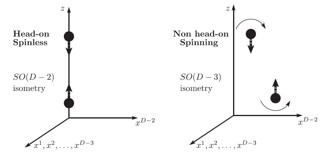
 -dimensional representation of head-on collisons for spinless BHs, with isometry group
 (left), and non-head-on collisons for BHs spinning in the orbital plane, with isometry
group
(left), and non-head-on collisons for BHs spinning in the orbital plane, with isometry
group  (right). Image reproduced with permission from
 We shall use the following conventions for indices. As before, Greek indices  cover all
spacetime dimensions and late upper case capital Latin indices
cover all
spacetime dimensions and late upper case capital Latin indices  cover the
  spatial dimensions, whereas late lower case Latin indices
  cover the three spatial
dimensions of the eventual computational domain. In addition, we introduce barred Greek indices
cover the three spatial
dimensions of the eventual computational domain. In addition, we introduce barred Greek indices
 which also include time, and early lower case Latin indices
  describing the
  spatial directions associated with the rotational symmetry. Under the
  splitting of spacetime dimensions, then, the coordinates
  decompose as
  .
When explicitly stated, we shall consider instead a
.
When explicitly stated, we shall consider instead a  splitting, e.g., with barred
Greek indices running from
splitting, e.g., with barred
Greek indices running from  to
to  , and early lower case Latin indices running from
  to
to
 .
.
6.2.1 Dimensional reduction by isometry
The idea of dimensional reduction had originally been developed by Geroch [347] for four-dimensional spacetimes possessing one Killing field as for example in the case of axisymmetry; for numerical applications see for example Refs. [535, 704, 722, 214]. The case of arbitrary spacetime dimensions and number of Killing vectors has been discussed in Refs. [210, 211].12 More recently, this idea has been used to develop a convenient formalism to perform NR simulations of BH dynamical systems in higher dimensions, with or
or  isometry [841*, 797*].
Comprehensive summaries of this approach are given in Refs. [835*, 791, 792].
isometry [841*, 797*].
Comprehensive summaries of this approach are given in Refs. [835*, 791, 792].
The starting point is the general  -dimensional spacetime metric written in coordinates adapted to the
symmetry
-dimensional spacetime metric written in coordinates adapted to the
symmetry

 and
and  represent a scale parameter and a coupling constant that will soon drop out and play no
role in the eventual spacetime reduction. We note that the metric (82*) is fully general in the same sense as
the spacetime metric in the ADM split discussed in Section 6.1.1.
represent a scale parameter and a coupling constant that will soon drop out and play no
role in the eventual spacetime reduction. We note that the metric (82*) is fully general in the same sense as
the spacetime metric in the ADM split discussed in Section 6.1.1.
The special case of a  (
( ) isometry admits
  Killing fields
  where
where  (
( ) stands for the number of extra dimensions. For
  , for instance,
there exist three Killing fields given in spherical coordinates by
, for instance,
there exist three Killing fields given in spherical coordinates by  ,
,  ,
,
 .
.
Killing’s equation  implies that

 describes a
  splitting in
the case of
splitting in
the case of  isometry, and a
  splitting in the case of
  isometry.
From these conditions, we draw the following conclusions: (i)  , where
  is the
metric on the
is the
metric on the  sphere with unit radius and
  is a free field; (ii)
  in adapted
coordinates; (iii)
in adapted
coordinates; (iii) ![[ξ(i),B ¯μ] = 0](article679x.gif) . We here remark an interesting consequence of the last property. Since, for
. We here remark an interesting consequence of the last property. Since, for
 , there exist no nontrivial vector fields on
  that commute with all Killing fields, all vector fields
 vanish; when, instead,
  (i.e., when
  , or
, or  for
for  isometry), this
conclusion can not be made. In this approach, as it has been developed up to now [841*, 797*, 796*], one
restricts to the
isometry), this
conclusion can not be made. In this approach, as it has been developed up to now [841*, 797*, 796*], one
restricts to the  case, and it is then possible to assume
  . Eq. (82*) then reduces to the
form13
. Eq. (82*) then reduces to the
form13

 in the case of
  isometry, and
 in the case of
  isometry.
As mentioned above, since the Einstein equations have to be implemented in a four-dimensional
NR code, we eventually have to perform a  splitting, even when the spacetime
isometry is
splitting, even when the spacetime
isometry is  . This means that the line element is (84*), with
  and
and
 . In this case, only a subset
  of the isometry is
manifest in the line element; the residual symmetry yields an extra relation among the components
of the isometry is
manifest in the line element; the residual symmetry yields an extra relation among the components
 . If the isometry group is
  , the line element is the same, but there is no extra
relation.
, the line element is the same, but there is no extra
relation.
A tedious but straightforward calculation [835] shows that the components of the  -dimensional Ricci
tensor can then be written as
-dimensional Ricci
tensor can then be written as
![R = {(D − 5) − e2ψ [(D − 4 )∂ ¯μψ∂ ψ + ¯∇ ¯μ∂ ψ ]}Ω , ab ¯μ ¯μ ab R ¯μa = 0, R ¯μ¯ν = ¯R ¯μν¯− (D − 4)(¯∇ ¯ν∂¯μψ + ∂¯μψ ∂¯νψ ), [ −2ψ ¯μ μ¯ ] R = ¯R + (D − 4) (D − 5)e − 2¯∇ ∂¯μψ − (D − 3)∂ ψ ∂¯μψ , (85 )](article702x.gif)
 ,
,  and
and  respectively denote the 3 + 1-dimensional Ricci tensor, Ricci scalar and
covariant derivative associated with the 3 + 1 metric
respectively denote the 3 + 1-dimensional Ricci tensor, Ricci scalar and
covariant derivative associated with the 3 + 1 metric  . The
. The  -dimensional vacuum Einstein
equations with cosmological constant
-dimensional vacuum Einstein
equations with cosmological constant  can then be formulated in terms of fields on a 3 + 1-dimensional
manifold
One important comment is in order at this stage. If we describe the three spatial dimensions in terms of
Cartesian coordinates
can then be formulated in terms of fields on a 3 + 1-dimensional
manifold
One important comment is in order at this stage. If we describe the three spatial dimensions in terms of
Cartesian coordinates ![R¯ = (D − 4)(¯∇ ∂ ψ − ∂ ψ ∂ ψ ) − Λ ¯g , (86 ) 2¯μψ¯ν[ ¯μ ν¯ ¯μ ¯μ¯μ ¯ν ] ¯μ¯ν e (D − 4 )∂ ψ∂μ¯ψ + ¯∇ ∂¯μψ − Λ = (D − 5). (87 )](article709x.gif)
 , one of these is now a quasi-radial coordinate. Without loss of generality,
we choose
, one of these is now a quasi-radial coordinate. Without loss of generality,
we choose  and the computational domain is given by
  ,
,  . In consequence of the radial
nature of the
. In consequence of the radial
nature of the  direction,
  at
at  . Numerical problems arising from this coordinate
singularity can be avoided by working instead with a rescaled version of the variable
. Numerical problems arising from this coordinate
singularity can be avoided by working instead with a rescaled version of the variable  . More
specifically, we also include the BSSN conformal factor
. More
specifically, we also include the BSSN conformal factor  in the redefinition and write
The BSSN version of the
in the redefinition and write
The BSSN version of the 
 -dimensional vacuum Einstein equations (86*), (87*) with
  in its
dimensionally reduced form on a 3 + 1 manifold is then given by Eqs. (60*) – (64*) with the following
modifications. (i) Upper-case capital indices
in its
dimensionally reduced form on a 3 + 1 manifold is then given by Eqs. (60*) – (64*) with the following
modifications. (i) Upper-case capital indices  are replaced with their lower case counterparts
 . (ii) The
  dimensional metric
  , Christoffel symbols
  , covariant
derivative
, covariant
derivative  , conformal factor
  and extrinsic curvature variables
  and
and  are replaced by the
 dimensional metric
  , the
, the  dimensional Christoffel symbols
  , the covariant derivative
  ,
as well as the conformal factor
,
as well as the conformal factor  ,
,  and
and  defined in analogy to Eq. (58*) with
  , i.e.
(iii) The extra dimensions manifest themselves as quasi-matter terms given by
Here,
, i.e.
(iii) The extra dimensions manifest themselves as quasi-matter terms given by
Here, 
![yy y 4π-(ρ-+-S-) = (D − 5)χ-&tidle;γ--ζ −-1-− 2D--−-7&tidle;γmn ∂ η ∂ χ − χ &tidle;Γ--+ D--−-6-χ-&tidle;γmn ∂ ζ ∂ ζ D − 4 ζ y2 4 ζ m n y 4 ζ2 m n 1 &tidle;γym ( χ ) KK K2 + --γ&tidle;mn (χ &tidle;Dm ∂nζ − ζD&tidle;m ∂nχ) + (D − 4)---- --∂mζ − ∂m χ − ----ζ − --- 2ζ y ζ ζ 3 1 &tidle;γym D − 1 ∂ χ ∂ χ ( K K )2 − -----∂m χ + ------&tidle;γmn -m----n--− (D − 5) --ζ + --- , (90 ) 2( y ) 4 [ χ ζ 3 8π χSTiFj K ζ K 1 2χ y y 1 χ -------- = − --- + --- A&tidle;ij + -- --(δ (j∂i)ζ − ζ&tidle;Γij) + --∂iχ ∂jχ − &tidle;Di∂jχ + --D&tidle;i ∂jζ D − 4 ζ 3 ( 2 yζ ) 2χ ] ζ 1 mn χ &tidle;γym χ TF + ---&tidle;γij&tidle;γ ∂n χ ∂m χ − --∂mζ − &tidle;γij----∂m χ − --2∂iζ ∂jζ (91 ) 2(χ ) ζ (y 2ζ ) 16-πji 2- y K-ζ ym &tidle; 2- Kζ- 1- 1- 2- D − 4 = y δ iζ − γ&tidle; Ami + ζ∂iK ζ − ζ χ ∂iχ + ζ∂iζ + 3∂iK ( ) − &tidle;γnm &tidle;Ami 1∂nζ − -1∂nχ . (92 ) ζ χ](article741x.gif)
 . The evolution of the field
  is determined by Eq. (87*) which in
terms of the BSSN variables becomes
It has been demonstrated in Ref. [841*] how all terms containing factors of
is determined by Eq. (87*) which in
terms of the BSSN variables becomes
It has been demonstrated in Ref. [841*] how all terms containing factors of ![2 βy ∂tζ = βm∂m ζ − 2αK ζ − -ζ∂m βm + 2 ζ--, (93 ) 3 y m 2- m βy- 1- γ&tidle;ym- ∂tK ζ = β ∂mK ζ − 3K ζ∂m β + 2y K ζ − 3 ζ(∂t − ℒ β)K − χζ y ∂m α [ yy ym − 1&tidle;γmn ∂ α (χ ∂ ζ − ζ∂ χ ) + α (5 − D )χ ζ&tidle;γ--−--1-+ (4 − D )χ &tidle;γ---∂ ζ 2 m n n y2 y m 2D − 7 &tidle;γym 6 − D χ 2D − 7 + -------ζ----∂m χ + --------&tidle;γmn ∂mζ ∂n ζ + -------&tidle;γmn ∂mζ ∂n χ 2 y 4 ζ 4 1 − D ζ mn K2ζ 2D − 5 D − 1 2 + -------γ&tidle; ∂m χ ∂nχ + (D − 6)--- + ------- KK ζ + ------ζK 4 χ ζ ] 3 9 1 mn &tidle;Γ y + 2&tidle;γ (ζ &tidle;Dm ∂n χ − χD&tidle;m ∂nζ) + χζ-y- . (94 )](article744x.gif)
 in the denominator can be
regularized using the symmetry properties of tensors and their derivatives across
in the denominator can be
regularized using the symmetry properties of tensors and their derivatives across  and assuming that
the spacetime does not contain a conical singularity.
and assuming that
the spacetime does not contain a conical singularity.
6.2.2 The cartoon method
The cartoon method has originally been developed in Ref. [25] for evolving axisymmetric four-dimensional spacetimes using an effectively two-dimensional spatial grid which employs ghostzones, i.e., a small number of extra gridpoints off the computational plane required for evaluating finite differences in the third spatial direction. Integration in time, however, is performed exclusively on the two-dimensional plane whereas the ghostzones are filled in after each timestep by appropriate interpolation of the fields in the plane and subsequent rotation of the solution using the axial spacetime symmetry. A version of this method has been applied to 5-dimensional spacetimes in Ref. [820*]. For arbitrary spacetime dimensions, however, even the relatively small number of ghostzones required in every extra dimension leads to a substantial increase in the computational resources; for fourth-order finite differencing, for example, four ghostzones are required in each extra dimension resulting in an increase of the computational domain by an overall factor . An elegant scheme to avoid
this difficulty while preserving all advantages of the cartoon method has been developed in
Ref. [630*] and is sometimes referred to as the modified cartoon method. This method has been
applied to
. An elegant scheme to avoid
this difficulty while preserving all advantages of the cartoon method has been developed in
Ref. [630*] and is sometimes referred to as the modified cartoon method. This method has been
applied to  dimensions in Refs. [700*, 512, 821] and we will discuss it now in more
detail.
dimensions in Refs. [700*, 512, 821] and we will discuss it now in more
detail.
Let us consider for illustrating this method a  -dimensional spacetime with
  symmetry and Cartesian coordinates
  , where
  .
Without loss of generality, the coordinates are chosen such that the
.
Without loss of generality, the coordinates are chosen such that the  symmetry
implies rotational symmetry in the planes spanned by each choice of two coordinates
from14
symmetry
implies rotational symmetry in the planes spanned by each choice of two coordinates
from14
 . The goal is to obtain a formulation of the
  -dimensional Einstein equations (60*) – (69*) with
 symmetry that can be evolved exclusively on the
  hyperplane. The tool employed for
this purpose is to use the spacetime symmetries in order to trade derivatives off the hyperplane, i.e., in the
hyperplane. The tool employed for
this purpose is to use the spacetime symmetries in order to trade derivatives off the hyperplane, i.e., in the
 directions, for derivatives inside the hyperplane. Furthermore, the symmetry implies relations between
the
directions, for derivatives inside the hyperplane. Furthermore, the symmetry implies relations between
the  -dimensional components of the BSSN variables.
These relations are obtained by applying a coordinate transformation from Cartesian to polar
coordinates in any of the two-dimensional planes spanned by  and
and  , where
  for any
particular choice of
for any
particular choice of 
 dimensions implies the existence of
  Killing vectors, one
for each plane with rotational symmetry. For each Killing vector
Killing vectors, one
for each plane with rotational symmetry. For each Killing vector  , the Lie derivative of the spacetime
metric vanishes. For the
, the Lie derivative of the spacetime
metric vanishes. For the  plane, in particular, the Killing vector field is
  and the Killing
condition is given by the simple relation
All ADM and BSSN variables are constructed from the spacetime metric and a straightforward
calculation demonstrates that the Lie derivatives along
and the Killing
condition is given by the simple relation
All ADM and BSSN variables are constructed from the spacetime metric and a straightforward
calculation demonstrates that the Lie derivatives along 
 of all these variables vanish. For
 , we can always choose the coordinates such that for
  ,
,  which implies the
vanishing of the BSSN variables
which implies the
vanishing of the BSSN variables  . The case of
  symmetry in
 dimensions is special in the same sense as already discussed in Section 6.2.1 and the
vanishing of
dimensions is special in the same sense as already discussed in Section 6.2.1 and the
vanishing of  does not in general hold. As before, we therefore consider in
  the
more restricted class of
the
more restricted class of  isometry which implies
  . Finally, the Cartesian
coordinates
. Finally, the Cartesian
coordinates  can always be chosen such that the diagonal metric components are equal,
We can now exploit these properties in order to trade derivatives in the desired manner. We shall illustrate
this for the second
can always be chosen such that the diagonal metric components are equal,
We can now exploit these properties in order to trade derivatives in the desired manner. We shall illustrate
this for the second 
 derivative of the
  component of a symmetric
  tensor density
 of weight
  which transforms under change of coordinates
  according to
Specifically, we consider the coordinate transformation (95*) where
according to
Specifically, we consider the coordinate transformation (95*) where 
 . In particular, this
transformation implies
and we can substitute
Inserting (100*) into (99*) and setting
. In particular, this
transformation implies
and we can substitute
Inserting (100*) into (99*) and setting 

 yields a lengthy expression involving derivatives of
  and
and
 with respect to
  and
and  . The latter vanish due to symmetry and we substitute for the
  derivatives using
This gives a lengthy expression relating the
derivatives using
This gives a lengthy expression relating the ![( ) [ ( ) ] ∂ S = ∂y-∂ + ∂w-∂ 𝒥 𝒲 ∂y-∂y-S + 2∂y-∂w-S + ∂w-∂w-S , ρ ρρ ∂ρ y ∂ρ w ∂ρ ∂ρ yy ∂ρ ∂ρ yw ∂ρ ∂ ρ ww ( ∂y ∂w ) [ ( ∂y ∂y ∂y ∂w ∂w ∂w ) ] ∂ ρSφφ = ---∂y + ---∂w 𝒥 𝒲 ------Syy + 2--- ---Syw + --- ---Sww . (101 ) ∂ρ ∂ρ ∂φ ∂φ ∂ φ ∂φ ∂φ ∂φ](article802x.gif)
 and
and  derivatives of
  . Finally, we recall that we
need these derivatives in the
. Finally, we recall that we
need these derivatives in the  hyperplane and therefore set
  . In order to obtain an expression
for the second
. In order to obtain an expression
for the second  derivative of
  , we first differentiate the expression with respect to
  and then
set
and then
set  . The final result is given by
Note that the density weight dropped out of this calculation, so that Eq. (102*) is valid for the BSSN
variables
. The final result is given by
Note that the density weight dropped out of this calculation, so that Eq. (102*) is valid for the BSSN
variables 
 and
and  as well.
Applying a similar procedure to all components of scalar, vector and symmetric tensor densities gives all
expressions necessary to trade derivatives off the  hyperplane for those inside it. We summarize the
expressions recalling our notation: a late Latin index,
hyperplane for those inside it. We summarize the
expressions recalling our notation: a late Latin index,  stands for either
  ,
,  or
or  whereas an early Latin index,
  represents any of the
  directions. For scalar, vector
and tensor fields
directions. For scalar, vector
and tensor fields  ,
,  and
and  we obtain
 -dimensional spacetimes with
  symmetry on a strictly three-dimensional computational
grid. We finally note that
symmetry on a strictly three-dimensional computational
grid. We finally note that  is a quasi-radial variable so that
  .
.
6.3 Initial data
In Section 6.1 we have discussed different ways of casting the Einstein equations into a form suitable for numerical simulations. At the start of Section 6, we have listed a number of additional ingredients that need to be included for a complete numerical study and physical analysis of BH spacetimes. We will now discuss the main choices used in practical computations to address these remaining items, starting with the initial conditions.As we have seen in Section 6.1, initial data to be used in time evolutions of the Einstein equations need to satisfy the Hamiltonian and momentum constraints (54*), (55*). A comprehensive overview of the approach to generate BH initial data is given by Cook’s Living Reviews article [224*]. Here we merely summarize the key concepts used in the construction of vacuum initial data, but discuss in some more detail how solutions to the constraint equations can be generated in the presence of specific matter fields that play an important role in the applications discussed in Section 7.
One obvious way to obtain constraint-satisfying initial data is to directly use analytical solutions to the
Einstein equations as for example the Schwarzschild solution in  in isotropic coordinates
![( ) ( ) 2 M − 2r 2 2 M 4[ 2 2 2 2 2 ] ds = − M--+-2r- dt + 1 + 2r- dr + r( d𝜃 + sin 𝜃d ϕ ) . (104 )](article831x.gif)
 non-spinning BHs at the moment of
time symmetry. In Cartesian coordinates, the Brill–Lindquist data generalized to arbitrary
non-spinning BHs at the moment of
time symmetry. In Cartesian coordinates, the Brill–Lindquist data generalized to arbitrary  are given by
where the summations over
are given by
where the summations over ∕2 A 4 K=1(x − x 0 )](article834x.gif)
 and
and  run over the number of BHs and the spatial coordinates,
respectively, and
run over the number of BHs and the spatial coordinates,
respectively, and  are parameters related to the mass of the
  -th BH through the surface area
 of the
  -dimensional sphere by
 ![μA = 16πM ∕[(D − 2 )ΩD − 2]](article841x.gif) . We remark that in the case
of a single BH, the Brill–Lindquist initial data (105*) reduce to the Schwarzschild spacetime in Cartesian,
isotropic coordinates (see Eq. (137*) in Section 6.7.1).
. We remark that in the case
of a single BH, the Brill–Lindquist initial data (105*) reduce to the Schwarzschild spacetime in Cartesian,
isotropic coordinates (see Eq. (137*) in Section 6.7.1).
A systematic way to generate solutions to the constraints describing BHs in  dimensions is
based on the York–Lichnerowicz split [515, 806, 807]. This split employs a conformal spatial metric defined
by
dimensions is
based on the York–Lichnerowicz split [515, 806, 807]. This split employs a conformal spatial metric defined
by  ; note that in contrast to the BSSN variable
  , in general
  . Applying a
conformal traceless split to the extrinsic curvature according to
. Applying a
conformal traceless split to the extrinsic curvature according to

 into a longitudinal and a transverse traceless part, the momentum
constraints simplify significantly; see [224*] for details as well as a discussion of the alternative
physical transverse-traceless split and conformal thin-sandwich decomposition [813]. The conformal
thin-sandwich approach, in particular, provides a method to generate initial data for the lapse and shift
which minimize the initial rate of change of the spatial metric, i.e., data in a quasi-equilibrium
configuration [225, 190].
into a longitudinal and a transverse traceless part, the momentum
constraints simplify significantly; see [224*] for details as well as a discussion of the alternative
physical transverse-traceless split and conformal thin-sandwich decomposition [813]. The conformal
thin-sandwich approach, in particular, provides a method to generate initial data for the lapse and shift
which minimize the initial rate of change of the spatial metric, i.e., data in a quasi-equilibrium
configuration [225, 190].
Under the further assumption of vanishing trace of the extrinsic curvature  , a flat
conformal metric
, a flat
conformal metric  , where
  describes a flat Euclidean space, and asymptotic flatness
 , the momentum constraint admits an analytic solution known as Bowen–York data [121*]
![3 [ k ] 3 ( l k l k ) A¯ij = 2r2-Pinj + Pjni − (fij − ninj)P nk + r3 𝜖kilS n nj + 𝜖kjlS n ni , (107 )](article852x.gif)
 ,
,  the unit radial vector and user-specified parameters
  ,
,  . By
calculating the momentum associated with the asymptotic translational and rotational Killing vectors
. By
calculating the momentum associated with the asymptotic translational and rotational Killing vectors  [811], one can show that
  and
and  represent the components of the total linear and angular
momentum of the initial hypersurface. The linearity of the momentum constraint further allows us to
superpose solutions
represent the components of the total linear and angular
momentum of the initial hypersurface. The linearity of the momentum constraint further allows us to
superpose solutions  of the type (107*) and the total linear momentum is merely obtained by
summing the individual
of the type (107*) and the total linear momentum is merely obtained by
summing the individual  . The total angular momentum is given by the sum of the individual
spins
. The total angular momentum is given by the sum of the individual
spins  plus an additional contribution representing the orbital angular momentum. For
the generalization of Misner data, it is necessary to construct inversion-symmetric solutions of
the type (107*) using the method of images [121, 224*]. Such a procedure is not required for
generalizing Brill–Lindquist data where a superposition of solutions
plus an additional contribution representing the orbital angular momentum. For
the generalization of Misner data, it is necessary to construct inversion-symmetric solutions of
the type (107*) using the method of images [121, 224*]. Such a procedure is not required for
generalizing Brill–Lindquist data where a superposition of solutions  of the type (107*) can
be used directly to calculate the extrinsic curvature from Eq. (106*) and insert the resulting
expressions into the vacuum Hamiltonian constraint given with the above listed simplifications by
where
of the type (107*) can
be used directly to calculate the extrinsic curvature from Eq. (106*) and insert the resulting
expressions into the vacuum Hamiltonian constraint given with the above listed simplifications by
where 
 is the Laplace operator associated with the flat metric
  . This elliptic equation is
commonly solved by decomposing
. This elliptic equation is
commonly solved by decomposing  into a Brill–Lindquist piece
  plus a regular piece
  , where
  denotes the location of the
  -th BH and
 a parameter that determines the BH mass and is sometimes referred to as the bare mass.
Brandt & Brügmann [126] have proven existence and uniqueness of
a parameter that determines the BH mass and is sometimes referred to as the bare mass.
Brandt & Brügmann [126] have proven existence and uniqueness of  regular solutions
 to Eq. (108*) and the resulting puncture data are the starting point of the majority of
numerical BH evolutions using the BSSN moving puncture technique. The simplest example
of this type of initial data is given by Schwarzschild’s solution in isotropic coordinates where
In particular, this solution admits the isometry
to Eq. (108*) and the resulting puncture data are the starting point of the majority of
numerical BH evolutions using the BSSN moving puncture technique. The simplest example
of this type of initial data is given by Schwarzschild’s solution in isotropic coordinates where
In particular, this solution admits the isometry 
 which leaves the coordinate sphere
 invariant, but maps the entire asymptotically flat spacetime
  into the interior and vice
versa. The solution, therefore, consists of 2 asymptotically flat regions connected by a “throat” and spatial
infinity of the far region is compactified into the single point
into the interior and vice
versa. The solution, therefore, consists of 2 asymptotically flat regions connected by a “throat” and spatial
infinity of the far region is compactified into the single point  which is commonly referred to as the
puncture. Originally, time evolutions of puncture initial data split the conformal factor, in analogy to the
initial-data construction, into a singular Brill–Lindquist contribution given by the
which is commonly referred to as the
puncture. Originally, time evolutions of puncture initial data split the conformal factor, in analogy to the
initial-data construction, into a singular Brill–Lindquist contribution given by the  in Eq. (109*) plus a
deviation
in Eq. (109*) plus a
deviation  that is regular everywhere; cf. Section IV B in [24*]. In this approach, the puncture
locations remain fixed on the computational domain. The simulations through inspiral and merger
by [159*, 65*], in contrast, evolve the entire conformal factor using gauge conditions that allow for the
puncture to move across the domain and are, therefore, often referred to as “moving puncture
evolutions”.
that is regular everywhere; cf. Section IV B in [24*]. In this approach, the puncture
locations remain fixed on the computational domain. The simulations through inspiral and merger
by [159*, 65*], in contrast, evolve the entire conformal factor using gauge conditions that allow for the
puncture to move across the domain and are, therefore, often referred to as “moving puncture
evolutions”.
In spite of its popularity, there remain a few caveats with puncture data that have inspired explorations
of alternative initial data. In particular, it has been shown that there exist no maximal, conformally
flat spatial slices of the Kerr spacetime [341, 756]. Constructing puncture data of a single BH
with non-zero Bowen–York parameter  will, therefore, inevitably result in a hypersurface
containing a BH plus some additional content which typically manifests itself in numerical
evolutions as spurious GWs, colloquially referred to as “junk radiation”. For rotation parameters
close to the limit of extremal Kerr BHs, the amount of spurious radiation rapidly increases
leading to an upper limit of the dimensionless spin parameter
will, therefore, inevitably result in a hypersurface
containing a BH plus some additional content which typically manifests itself in numerical
evolutions as spurious GWs, colloquially referred to as “junk radiation”. For rotation parameters
close to the limit of extremal Kerr BHs, the amount of spurious radiation rapidly increases
leading to an upper limit of the dimensionless spin parameter  for conformally flat
Bowen–York-type data [226, 237, 238, 527*]; BH initial data of Bowen–York type with a spin
parameter above this value rapidly relax to rotating BHs with spin
for conformally flat
Bowen–York-type data [226, 237, 238, 527*]; BH initial data of Bowen–York type with a spin
parameter above this value rapidly relax to rotating BHs with spin  , probably through
absorption of some fraction of the spurious radiation. This limit has been overcome [527, 528]
by instead constructing initial data with an extended version of the conformal thin-sandwich
method using superposed Kerr–Schild BHs [467]. In an alternative approach, most of the above
outlined puncture method is applied but using a non-flat conformal metric; see for instance
[493, 391].
, probably through
absorption of some fraction of the spurious radiation. This limit has been overcome [527, 528]
by instead constructing initial data with an extended version of the conformal thin-sandwich
method using superposed Kerr–Schild BHs [467]. In an alternative approach, most of the above
outlined puncture method is applied but using a non-flat conformal metric; see for instance
[493, 391].
In practice, puncture data are the method-of-choice for most evolutions performed with the BSSN-moving-puncture
technique15
whereas GHG evolution schemes commonly start from conformal thin-sandwich data using
either conformally flat or Kerr–Schild background data. Alternatively to both these approaches,
initial data containing scalar fields which rapidly collapse to one or more BHs has also been
employed [629*].
The constraint equations in the presence of matter become more complex. A simple procedure can however be used to yield analytic solutions to the initial data problem in the presence of minimally coupled scalar fields [588*, 586*]. Although in general the constraints (54*) – (55*) have to be solved numerically, there is a large class of analytic or semi-analytic initial data for the Einstein equations extended to include scalar fields. The construction of constraint-satisfying initial data starts from a conformal transformation of the ADM variables [224]
which can be used to re-write the constraints as Here,
![1 1 2 5 1 ij − 7 [ i ∗ 4( ∗ 2 ∗ )] ℋ = △¯ψ − 8R¯ψ − 12K ψ + 8 ¯A ¯Aijψ + π ψ D¯ Φ D¯i Φ + ψ Π Π + μ SΦ Φ , (112 ) ℳ = D¯ A¯j − 2ψ6D¯ K − 4 πψ6 (Π∗D¯ Φ + Π ¯D Φ ∗). (113 ) i j i 3 i i i](article886x.gif)
 ,
,  and
and  denote the conformal covariant derivative and Ricci scalar and
  is a
time reduction variable defined in (78*).
is a
time reduction variable defined in (78*).
Take for simplicity a single, non-rotating BH surrounded by a scalar field (more general cases are studied
in Ref. [588*, 586*]). If we adopt the maximal slicing condition  and set
  , then the
momentum constraint is immediately satisfied, and one is left with the the Hamiltonian constraint, which
for conformal flatness, i.e.,
, then the
momentum constraint is immediately satisfied, and one is left with the the Hamiltonian constraint, which
for conformal flatness, i.e.,  reads
reads
![[ 2 ] 1--∂- 2-∂- ---1---∂-- -∂- ---1-----∂-- 5 ∗ △ flat ψ = r2∂r r ∂r + r2sin𝜃 ∂𝜃 sin 𝜃∂ 𝜃 + r2sin2𝜃 ∂Φ2 ψ = − πψ ΠΠ . (114 )](article894x.gif)

 , or in other words, by projecting
  onto spherical harmonics
  , the above equation reduces to a single second-order, ordinary
differential equation. Thus, the complex problem of finding appropriate initial data for massive
scalar fields was reduced to an almost trivial problem, which admits some interesting analytical
solutions [588*, 586*]. Let us focus for definiteness on spherically symmetric solutions (we refer
the reader to Ref. [588*, 586*] for the general case), by taking a Gaussian-type solution ansatz,
where
, the above equation reduces to a single second-order, ordinary
differential equation. Thus, the complex problem of finding appropriate initial data for massive
scalar fields was reduced to an almost trivial problem, which admits some interesting analytical
solutions [588*, 586*]. Let us focus for definiteness on spherically symmetric solutions (we refer
the reader to Ref. [588*, 586*] for the general case), by taking a Gaussian-type solution ansatz,
where 
 is the scalar field amplitude and
  and
and  are the location of the center of the Gaussian
and its width. By solving Eq. (117*), we obtain the only non-vanishing component of
are the location of the center of the Gaussian
and its width. By solving Eq. (117*), we obtain the only non-vanishing component of  where we have imposed that
 ![2 [ ( √ -- ) ] 2 u = A2 w-[w--−--4r√0(r −-r0)] erf --2(r −-r0) − 1 − A2 r0√w--e−2(r− r0)2∕w2, (119 ) 00 00 16 2 w 008 π](article905x.gif)
 at infinity. Other solutions can be obtained by adding a constant to
(119*).
at infinity. Other solutions can be obtained by adding a constant to
(119*).
6.4 Gauge conditions
We have seen in Section 6.1, that the Einstein equations do not make any predictions about the gauge
functions; the ADM equations leave lapse  and shift
  unspecified and the GHG equations make no
predictions about the source functions
unspecified and the GHG equations make no
predictions about the source functions  . Instead, these functions can be freely specified by the user and
represent the coordinate or gauge-invariance of the theory of GR. Whereas the physical properties of a
spacetime remain unchanged under gauge transformations, the performance of numerical evolution schemes
depends sensitively on the gauge choice. It is well-known, for example, that evolutions of the Schwarzschild
spacetime employing geodesic slicing
. Instead, these functions can be freely specified by the user and
represent the coordinate or gauge-invariance of the theory of GR. Whereas the physical properties of a
spacetime remain unchanged under gauge transformations, the performance of numerical evolution schemes
depends sensitively on the gauge choice. It is well-known, for example, that evolutions of the Schwarzschild
spacetime employing geodesic slicing  and vanishing shift
  inevitably reach a
hypersurface containing the BH singularity after a coordinate time interval
inevitably reach a
hypersurface containing the BH singularity after a coordinate time interval  [709];
computers respond to singular functions with non-assigned numbers which rapidly swamp the entire
computational domain and render further evolution in time practically useless. This problem
can be avoided by controlling the lapse function such that the evolution in proper time slows
down in the vicinity of singular points in the spacetime [312]. Such slicing conditions are called
singularity avoiding and have been studied systematically in the form of the Bona-Massó
family of slicing conditions [116]; see also [343, 20]. A potential problem arising from the use
of singularity avoiding slicing is the different progress in proper time in different regions of
the computational domain resulting in a phenomenon often referred to as “grid stretching” or
“slice stretching” which can be compensated with suitable non-zero choices for the shift vector
[24*].
[709];
computers respond to singular functions with non-assigned numbers which rapidly swamp the entire
computational domain and render further evolution in time practically useless. This problem
can be avoided by controlling the lapse function such that the evolution in proper time slows
down in the vicinity of singular points in the spacetime [312]. Such slicing conditions are called
singularity avoiding and have been studied systematically in the form of the Bona-Massó
family of slicing conditions [116]; see also [343, 20]. A potential problem arising from the use
of singularity avoiding slicing is the different progress in proper time in different regions of
the computational domain resulting in a phenomenon often referred to as “grid stretching” or
“slice stretching” which can be compensated with suitable non-zero choices for the shift vector
[24*].
The particular coordinate conditions used with great success in the BSSN-based moving puncture
approach [159, 65] in  dimensions are variants of the “1+log” slicing and “
 -driver” shift
condition [24]
-driver” shift
condition [24]
 introduced here is an auxiliary variable to write the second-order-in-time
equation for the shift vector as a first-order system and has no relation with the variable of the same name
introduced in Eq. (82*). The “damping” factor
introduced here is an auxiliary variable to write the second-order-in-time
equation for the shift vector as a first-order system and has no relation with the variable of the same name
introduced in Eq. (82*). The “damping” factor  in Eq. (122*) is specified either as a constant, a
function depending on the coordinates
in Eq. (122*) is specified either as a constant, a
function depending on the coordinates  and BH parameters [683], a function of the BSSN
variables [559, 560], or evolved as an independent variable [29]. A first-order-in-time evolution
equation for
and BH parameters [683], a function of the BSSN
variables [559, 560], or evolved as an independent variable [29]. A first-order-in-time evolution
equation for  has been suggested in [758] which results from integration of Eqs. (121*), (122*)
Some NR codes omit the advection derivatives of the form
has been suggested in [758] which results from integration of Eqs. (121*), (122*)
Some NR codes omit the advection derivatives of the form 
 in Eqs. (120*) – (123*). Long-term stable
numerical simulations of BHs in higher dimensions require modifications in the coefficients in
Eqs. (120*) – (123*) [700*] and/or the addition of extra terms [841*]. Reference [313] recently suggested a
modification of Eq. (120*) for the lapse function
in Eqs. (120*) – (123*). Long-term stable
numerical simulations of BHs in higher dimensions require modifications in the coefficients in
Eqs. (120*) – (123*) [700*] and/or the addition of extra terms [841*]. Reference [313] recently suggested a
modification of Eq. (120*) for the lapse function  that significantly reduces noise generated by a sharp
initial gauge wave pulse as it crosses mesh refinement boundaries.
that significantly reduces noise generated by a sharp
initial gauge wave pulse as it crosses mesh refinement boundaries.
BH simulations with the GHG formulation employ a wider range of coordinate conditions. For example,
Pretorius’ breakthrough evolutions [629*] set  and
and

 ,
,  ,
,  where
where  denotes the mass of a single BH. An
alternative choice used with great success in long binary BH inspiral simulations [735] sets
denotes the mass of a single BH. An
alternative choice used with great success in long binary BH inspiral simulations [735] sets  such that
the dynamics are minimized at early stages of the evolution, gradually changes to harmonic
gauge
such that
the dynamics are minimized at early stages of the evolution, gradually changes to harmonic
gauge  during the binary inspiral and uses a damped harmonic gauge near merger
where
during the binary inspiral and uses a damped harmonic gauge near merger
where ![[ ( √ -) ]2[ ( √ -) ] H α = μ0 ln --γ- ln --γ- n α − α −1gαm βm , (125 ) α α](article931x.gif)
 is a free parameter. We note in this context that for
  , the GHG source functions
  are related to the ADM lapse and shift functions through [630*]
6.5 Discretization of the equations
In the previous sections, we have derived formulations of the Einstein equations in the form of an IBVP. Given an initial snapshot of the physical system under consideration, the evolution equations, as for example in the form of the BSSN equations (60*) – (64*), then predict the evolution of the system in time. These evolution equations take the form of a set of nonlinear partial differential equations which relate a number of grid variables and their time and spatial derivatives. Computers, on the other hand, exclusively operate with (large sets of) numbers and for a numerical simulation we need to translate the differential equations into expressions relating arrays of numbers.The common methods to implement this discretization of the equations are finite differencing, the finite element, finite volume and spectral methods. Finite element and volume methods are popular choices in various computational applications, but have as yet not been applied to time evolutions of BH spacetimes. Spectral methods provide a particularly efficient and accurate approach for numerical modelling provided the functions do not develop discontinuities. Even though BH spacetimes contain singularities, the use of singularity excision provides a tool to remove these from the computational domain. This approach has been used with great success in the SpEC code to evolve inspiralling and merging BH binaries with very high accuracy; see, e.g., [122, 220, 526]. Spectral methods have also been used successfully for the modelling of spacetimes with high degrees of symmetry [205, 206, 207*] and play an important role in the construction of initial data [39*, 38, 836*]. An indepth discussion of spectral methods is given in the Living Reviews article [365]. The main advantage of finite differencing methods is their comparative simplicity. Furthermore, they have proved very robust in the modelling of rather extreme BH configurations as for example BHs colliding near the speed of light [719*, 587*, 716*] or binaries with mass ratios up to 1 : 100 [525, 523, 718].
Mesh refinement and domain decomposition:
BH spacetimes often involve lengthscales that differ by orders of magnitude. The BH horizon extends over lengths of the order where
where  is the mass of the
BH. Inspiralling BH binaries, on the other hand, emit GWs with wavelengths of
is the mass of the
BH. Inspiralling BH binaries, on the other hand, emit GWs with wavelengths of  .
Furthermore, GWs are rigorously defined only at infinity. In practice, wave extraction is often
performed at finite radii but these need to be large enough to ensure that systematic errors are
small. In order to accomodate accurate wave extraction, computational domains used for the
modelling of asymptotically flat BH spacetimes typically have a size of
.
Furthermore, GWs are rigorously defined only at infinity. In practice, wave extraction is often
performed at finite radii but these need to be large enough to ensure that systematic errors are
small. In order to accomodate accurate wave extraction, computational domains used for the
modelling of asymptotically flat BH spacetimes typically have a size of  . With present
computational infrastructure it is not possible to evolve such large domains with a uniform,
high resolution that is sufficient to accurately model the steep profiles arising near the BH
horizon. The solution to this difficulty is the use of mesh refinement, i.e., a grid resolution that
depends on the location in space and may also vary in time. The use of mesh refinement in BH
modelling is simplified by the remarkably rigid nature of BHs which rarely exhibit complicated
structure beyond some mild deformation of a sphere. The requirements of increased resolution are,
therefore, simpler to implement than, say, in the modelling of airplanes or helicopters. In BH
spacetimes the grid resolution must be highest near the BH horizon and it decreases gradually at
larger and larger distances from the BH. In terms of the internal book-keeping, this allows
for a particularly efficient manner to arrange regions of refinement which is often referred to
as moving boxes. A set of nested boxes with outwardly decreasing resolution is centered on
each BH of the spacetime and follows the BH motion. These sets of boxes are immersed in
one or more common boxes which are large enough to accomodate those centered on the BHs.
As the BHs approach each other, boxes originally centered on the BHs merge into one and
become part of the common-box hierarchy. A snapshot of such moving boxes is displayed in
Figure 4*.
. With present
computational infrastructure it is not possible to evolve such large domains with a uniform,
high resolution that is sufficient to accurately model the steep profiles arising near the BH
horizon. The solution to this difficulty is the use of mesh refinement, i.e., a grid resolution that
depends on the location in space and may also vary in time. The use of mesh refinement in BH
modelling is simplified by the remarkably rigid nature of BHs which rarely exhibit complicated
structure beyond some mild deformation of a sphere. The requirements of increased resolution are,
therefore, simpler to implement than, say, in the modelling of airplanes or helicopters. In BH
spacetimes the grid resolution must be highest near the BH horizon and it decreases gradually at
larger and larger distances from the BH. In terms of the internal book-keeping, this allows
for a particularly efficient manner to arrange regions of refinement which is often referred to
as moving boxes. A set of nested boxes with outwardly decreasing resolution is centered on
each BH of the spacetime and follows the BH motion. These sets of boxes are immersed in
one or more common boxes which are large enough to accomodate those centered on the BHs.
As the BHs approach each other, boxes originally centered on the BHs merge into one and
become part of the common-box hierarchy. A snapshot of such moving boxes is displayed in
Figure 4*.
Mesh refinement in NR has been pioneered by Choptuik in his seminal study on critical phenomena in the collapse of scalar fields [212*]. The first application of mesh refinement to the evolution of BH binaries was performed by Brügmann [140*]. There exists a variety of mesh refinement packages available for use in NR including Bam [140], Had [384], Pamr/Amrd [754], Paramesh [534], Samrai [672] and the Carpet [684*, 184] package integrated into the Cactus Computational Toolkit [155]. For additional information on Cactus see also the Einstein Toolkit webpage [300] and the lecture notes [840]. A particular mesh-refinement algorithm used for many BH applications is the Berger–Oliger [90] scheme where coarse and fine levels communicate through interpolation in the form of the prolongation and restriction operation; see [684] for details. Alternatively, the different lengthscales can be handled efficiently through the use of multiple domains of different shapes. Communication between the individual subdomains is performed either through overlaps or directly at the boundary for touching domains. Details of this domain decomposition can be found in [618, 146] and references therein.
6.6 Boundary conditions
In NR, we typically encounter two types of physical boundaries, (i) inner boundaries due to the treatment of spacetime singularities in BH solutions and (ii) the outer boundary either at infinite distance from the strong-field sources or, in the form of an approximation to this scenario, at the outer edge of the computational domain at large but finite distances.
Singularity excision:
BH spacetimes generically contain singularities, either physical singularities with a divergent Ricci scalar or coordinate singularities where the spacetime curvature is well behaved but some tensor components approach zero or inifinite values. In the case of the Schwarzschild solution in Schwarzschild coordinates, for example, corresponds to a physical singularity
whereas the singular behaviour of the metric components
corresponds to a physical singularity
whereas the singular behaviour of the metric components  and
and  at
at  merely
reflects the unsuitable nature of the coordinates as
merely
reflects the unsuitable nature of the coordinates as  and can be cured, for example, by
transforming to Kruskal–Szekeres coordinates; cf. for example Chapter 7 in Ref. [186]. Both
types of singularities give rise to trouble in the numerical modelling of spacetimes because
computers only handle finite numbers. Some control is available in the form of gauge conditions
as discussed in Section 6.4; the evolution of proper time is slowed down when the evolution
gets close to a singularity. In general, however, BH singularities require some special numerical
treatment.
and can be cured, for example, by
transforming to Kruskal–Szekeres coordinates; cf. for example Chapter 7 in Ref. [186]. Both
types of singularities give rise to trouble in the numerical modelling of spacetimes because
computers only handle finite numbers. Some control is available in the form of gauge conditions
as discussed in Section 6.4; the evolution of proper time is slowed down when the evolution
gets close to a singularity. In general, however, BH singularities require some special numerical
treatment.
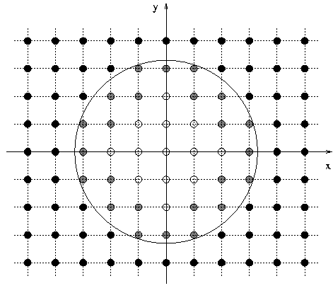
Such a treatment is most commonly achieved in the form of singularity or BH excision originally suggested by Unruh as quoted in [746]. According to Penrose’s cosmic censorship conjecture, a spacetime singularity should be cloaked inside an event horizon and the spacetime region outside the event horizon is causally disconnected from the dynamics inside (see Section 3.2.1). The excision technique is based on the corresponding assumption that the numerical treatment of the spacetime inside the horizon has no causal effect on the exterior. In particular, excising a finite region around the singularity but within the horizon should leave the exterior spacetime unaffected. This is illustrated in Figure 5* where the excision region is represented by small white circles which are excluded from the numerical evolution. Regular grid points, represented in the figure by black circles, on the other hand are evolved normally. As we have seen in the previous section, the numerical evolution in time of functions at a particular grid point typically requires information from neighbouring grid points. The updating of variables at regular points, therefore, requires data on the excision boundary represented in Figure 5* by gray circles. Inside the BH horizon, represented by the large circle in the figure, however, information can only propagate inwards, so that the variables on the excision boundary can be obtained through use of sideways derivative operators (e.g., [630]), extrapolation (e.g., [703, 723*]) or regular update with spectral methods (e.g., [677, 678*]). Singularity excision has been used with great success in many numerical BH evolutions [23, 723, 721*, 629*, 678, 70*, 418].
Quite remarkably, the moving puncture method for evolving BHs does not employ any such specific numerical treatment near BH singularities, but instead applies the same evolution procedure for points arbitrarily close to singularities as for points far away and appears “to get away with it”. In view of the remarkable success of the moving puncture method, various authors have explored the behaviour of the puncture singularity in the case of a single Schwarzschild BH [392, 136, 137, 390, 138*, 264]. Initially, the puncture represents spatial infinity on the other side of the wormhole geometry compactified into a single point. Under numerical evolution using moving puncture gauge conditions, however, the region immediately around this singularity rapidly evolves into a so-called trumpet geometry which is partially covered by the numerical grid to an extent that depends on the numerical resolution; cf. Figure 1 in [138]. In practice, the singularity falls through the inevitably finite resolution of the computational grid which thus facilitates a natural excision of the spacetime singularity without the need of any special numerical treatment.
Outer boundary:
Most physical scenarios of interest for NR involve spatial domains of infinite extent and there arises the question how these may be accomodated inside the finite memory of a computer system. Probably the most elegant and rigorous method is to apply a spatial compactification, i.e., a coordinate transformation that maps the entire domain including spatial infinity to a finite coordinate range. Such compactification is best achieved in characteristic formulations of the Einstein equations where the spacetime foliation in terms of ingoing and/or outgoing light cones may ensure adequate resolution of in- or outgoing radiation throughout the entire domain. In principle, such a compactification can also be implemented in Cauchy-type formulations, but here it typically leads to an increasing blueshift of radiative signals as they propagate towards spatial infinity. As a consequence, any discretization method applied will eventually fail to resolve the propagating features. This approach has been used in Pretorius’ breakthrough [629] and the effective damping of radiative signals at large distances through underresolving them approximates a no-ingoing-radiation boundary condition. An intriguing alternative consists in using instead a space-time slicing of asymptotically null hypersurfaces which play a key role in the conformal field equations [328]. To our knowledge, this method has not yet been applied successfully to BH simulations in either astrophysical problems or simulations of the type reviewed here, but may well merit more study in the future. The vast majority of Cauchy-based NR applications instead resort to an approximative treatment where the infinite spatial domain is truncated and modeled as a compact domain with “suitable” outer boundary conditions. Ideally, the boundary conditions would satisfy the following requirements [651*]: They (i) ensure well posedness of the IBVP, (ii) are compatible with the constraint equations, and (iii) correctly represent the physical conditions, which in almost all practical applications means that they control or minimize the ingoing gravitational radiation.Boundary conditions meeting these requirements at least partially have been studied most extensively for the harmonic or generalized harmonic formulation of the Einstein equations [492, 651, 58, 652*, 665].
For the BSSN system, such boundary conditions have as yet not been identified and practical
applications commonly apply outgoing radiation or Sommerfeld boundary conditions, which are an
approximation in this context, where they are applied at large but finite distances from the strong-field
region. Let us assume, for this purpose, that a given grid variable  asymptotes to a constant background
value
asymptotes to a constant background
value  in the limit of large
  and contains a leading order deviation
  from this value,
where
from this value,
where  remains finite as
  , and
, and  is a constant positive integer number. For
  , we
therefore have
, we
therefore have

 , which translates into the following conditon for the grid variable
  where
where 
 denote Cartesian coordinates. Because information only propagates outwards, the spatial
derivative
denote Cartesian coordinates. Because information only propagates outwards, the spatial
derivative  is evaluated using a one-sided stencil. This method is straightforwardly generalized to
asymptotically expanding cosmological spacetimes of dS type containing BHs; cf. Eq. (9) in Ref. [837*].
Even though this approximation appears to work rather (one might be tempted to say surprisingly) well in
practice [652], it is important to bear in mind the following caveats. (i) The number of conditions
imposed in this way exceeds the number of ingoing characteristics calling into question the
well-posedness of the resulting system. (ii) Sommerfeld conditions are not constraint satisfying
which leads to systematic errors that do not converge away as resolution is increased. (iii) Some
spurious reflections of gravitational waves may occur, especially when applied at too small radii.
These potential difficulties of BSSN evolutions have motivated studies of generalizing the BSSN
system, in particular the conformal Z4 formulations discussed in Section 6.1.5 which accomodate
constraint preserving boundary conditions which facilitate control of the ingoing gravitational
radiation [428].
is evaluated using a one-sided stencil. This method is straightforwardly generalized to
asymptotically expanding cosmological spacetimes of dS type containing BHs; cf. Eq. (9) in Ref. [837*].
Even though this approximation appears to work rather (one might be tempted to say surprisingly) well in
practice [652], it is important to bear in mind the following caveats. (i) The number of conditions
imposed in this way exceeds the number of ingoing characteristics calling into question the
well-posedness of the resulting system. (ii) Sommerfeld conditions are not constraint satisfying
which leads to systematic errors that do not converge away as resolution is increased. (iii) Some
spurious reflections of gravitational waves may occur, especially when applied at too small radii.
These potential difficulties of BSSN evolutions have motivated studies of generalizing the BSSN
system, in particular the conformal Z4 formulations discussed in Section 6.1.5 which accomodate
constraint preserving boundary conditions which facilitate control of the ingoing gravitational
radiation [428].
In asymptotically AdS spacetimes, the outer boundary represents a more challenging problem and the
difficulties just discussed are likely to impact numerical simulations more severely if not handled
appropriately. This is largely a consequence of the singular behaviour of the AdS metric even in the absence
of a BH or any matter sources. The AdS metric (see Section 3.3.1) is the maximally symmetric solution to
the Einstein equations (39*) with  and
and  . This solution can be represented by the
hyperboloid
. This solution can be represented by the
hyperboloid  embedded in a flat
  -dimensional spacetime with
metric
-dimensional spacetime with
metric  It can be represented in global coordinates, as

 and
and  (by unwrapping the cylindrical
time direction, the range of the time coordinate is often extended to
(by unwrapping the cylindrical
time direction, the range of the time coordinate is often extended to  ), or in the Poincarè
coordinates:
with
), or in the Poincarè
coordinates:
with ![[ ] 2 D∑−2 ds2 = L-- − dt2 + dz2 + (dxi)2 , (131 ) z2 i=1](article970x.gif)
 . It can be shown that Poincaré coordinates only cover half the hyperboloid and that
the other half corresponds to
. It can be shown that Poincaré coordinates only cover half the hyperboloid and that
the other half corresponds to  [81].
[81].
Clearly, both the global (130*) and the Poincaré (131*) versions of the AdS metric become singular at
their respective outer boundaries  or
or  . The induced metric at infinity is therefore only
defined up to a conformal rescaling. This remaining freedom manifests itself in the boundary topology of the
global and Poincaré metrics which, respecitvely, become in the limit
. The induced metric at infinity is therefore only
defined up to a conformal rescaling. This remaining freedom manifests itself in the boundary topology of the
global and Poincaré metrics which, respecitvely, become in the limit  and
and 

 in the former and
  in the latter
case.
in the latter
case.
The boundary treatment inside a numerical modelling of asymptotically AdS spacetimes needs to take
care of the singular nature of the metric. In practice, this is achieved through some form of regularization
which makes use of the fact that the singular piece of an asymptotically AdS spacetime is known in analytic
form, e.g., through Eqs. (130*) or (131*). In Ref. [70*] the spacetime metric is decomposed into an analytically
known AdS part plus a deviation which is regular at infinity. In this approach, particular care needs
to be taken of the gauge conditions to ensure that the coordinates remain compatible with
this decomposition throughout the simulation. An alternative approach consists in factoring
out appropriate factors involving the bulk coordinate as for example the term  in the
denominator on the right-hand side of Eq. (130*). This method is employed in several recent
works [207*, 415, 108*].
in the
denominator on the right-hand side of Eq. (130*). This method is employed in several recent
works [207*, 415, 108*].
We finally note that the boundary plays an active role in AdS spacetimes. The visualization of the AdS spacetime in the form of a Penrose diagram demonstrates that it is not globally hyperbolic, i.e., there exists no Cauchy surface on which initial data can be specified in such a way that the entire future of the spacetime is uniquely determined. This is in marked contrast to the Minkowski spacetime. Put in other words, the outer boundary of asymptotically flat spacetimes is represented in a Penrose diagram by a null surface such that information cannot propagate from infinity into the interior spacetime. In contrast, the outer boundary of asymptotically AdS spacetimes is timelike and, hence, the outer boundary actively influences the evolution of the interior. The specification of boundary conditions in NR applications to the gauge/gravity duality or AdS/CFT correspondence therefore reflects part of the description of the physical system under study; cf. Section 7.8.
6.7 Diagnostics
Once we have numerically generated a spacetime, there still remains the question of how to extract physical information from the large chunk of numbers the computer has written to the hard drive. This analysis of the data faces two main problems in NR applications, (i) the gauge or coordinate dependence of the results and (ii) the fact that many quantities we are familiar with from Newtonian physics are hard or not even possible to define in a rigorous fashion in GR. In spite of these difficulties, a number of valuable diagnostic tools have been developed and the purpose of this section is to review how these are extracted.The physical information is often most conveniently calculated from the ADM variables and we assume for
this discussion that a numerical solution is available in the form of the ADM variables  ,
,  ,
,  and
and  . Even if the time evolution has been performed using other variables as for example the BSSN or
GHG variables the conversion between these and their ADM counterparts according to Eq. (58*) or (43*) is
straightforward.
. Even if the time evolution has been performed using other variables as for example the BSSN or
GHG variables the conversion between these and their ADM counterparts according to Eq. (58*) or (43*) is
straightforward.
One evident diagnostic directly arises from the structure of the Einstein equations where the number of equations exceeds the number of free variables; cf. the discussion following Eq. (55*). Most numerical applications employ “free evolutions” where the evolution equations are used for updating the grid variables. The constraints are thus not directly used in the numerical evolution but need to be satisfied by any solution to the Einstein equations. A convergence analysis of the constraints (see for example Figure 3 in Ref. [714]) then provides an important consistency check of the simulations.
Before reviewing the extraction of physical information from a numerical simulation, we note a potential
subtlety arising from the convention used for Newton’s constant in higher-dimensional spacetimes. We wrote
the Einstein equations in the form (39*) and chose units where  and
and  . This implies that the
Einstein equations have the form
. This implies that the
Einstein equations have the form  for all spacetime dimensionalities
(here and in Section 6.7.1 we explicitly keep
for all spacetime dimensionalities
(here and in Section 6.7.1 we explicitly keep  in the equations). As we shall see below,
with this convention the Schwarzschild radius of a static BH in
in the equations). As we shall see below,
with this convention the Schwarzschild radius of a static BH in  dimensions is given by

 denotes the area of the unit
  sphere.
6.7.1 Global quantities and horizons
For spacetimes described by a metric that is asymptotically flat and time independent, the total mass-energy and linear momentum are given by the ADM mass and ADM momentum, respectively. These quantities arise from boundary terms in the Hamiltonian of GR and were derived by Arnowitt, Deser & Misner [47] in their canonical analysis of the theory. They are given in terms of the ADM variables by Here, the spatial tensor components
 and
and  are assumed to be given in Cartesian coordinates,
 is the outgoing unit vector normal to the area element
  of the
  sphere and
 . The above integral is defined only for a restricted class of coordinate systems, known
as asymptotic Euclidian coordinates for which the metric components are required to be of the form
. The above integral is defined only for a restricted class of coordinate systems, known
as asymptotic Euclidian coordinates for which the metric components are required to be of the form
 . Under a more restrictive set of assumptions about the fall-off behaviour of the metric
and extrinsic curvature components (see Sections 7.5.1 and 7.5.2 in [364*] and references therein for
a detailed discussion), one can also derive an expression for the global angular momentum
where
. Under a more restrictive set of assumptions about the fall-off behaviour of the metric
and extrinsic curvature components (see Sections 7.5.1 and 7.5.2 in [364*] and references therein for
a detailed discussion), one can also derive an expression for the global angular momentum
where 
 are the Killing vector fields associated with the asymptotic rotational symmetry given, in
 , by
, by  ,
,  and
and  . For a more-in-depth
discussion of the ADM mass and momentum as well as the conditions required for the definition of the
angular momentum the reader is referred to Section 7 of [364*]. Expressions for
. For a more-in-depth
discussion of the ADM mass and momentum as well as the conditions required for the definition of the
angular momentum the reader is referred to Section 7 of [364*]. Expressions for  ,
,  and
and  can
also be derived in more general (curvilinear) coordinate systems as long as the metric approaches the
flat-space form in those curvilinear coordinates at an appropriate rate; see, e.g., Section 7 in [364] for a
detailed review.
can
also be derived in more general (curvilinear) coordinate systems as long as the metric approaches the
flat-space form in those curvilinear coordinates at an appropriate rate; see, e.g., Section 7 in [364] for a
detailed review.
As an example, we calculate the ADM mass of the  -dimensional Schwarzschild BH in Cartesian,
isotropic coordinates
-dimensional Schwarzschild BH in Cartesian,
isotropic coordinates  described by the spatial metric

 . A straightforward calculation shows that
so that (since
. A straightforward calculation shows that
so that (since 
 )
where we have used the fact that in the limit
)
where we have used the fact that in the limit 
 we can raise and lower indices with the Euclidean
metric
we can raise and lower indices with the Euclidean
metric  and
and  . From Eq. (134*) we thus obtain
The Schwarzschild radius in areal coordinates is given by
. From Eq. (134*) we thus obtain
The Schwarzschild radius in areal coordinates is given by 
 and we have recovered
Eq. (133*).
and we have recovered
Eq. (133*).
The event horizon is defined as the boundary between points in the spacetime from which null geodesics
can escape to infinity and points from which they cannot. The event horizon is therefore by definition a
concept that depends on the entire spacetime. In the context of numerical simulations, this implies that an
event horizon can only be computed if information about the entire spacetime is stored which results in
large data sets even by contemporary standards. Nevertheless, event horizon finders have been developed in
Refs. [278, 223]. For many purposes, however, it is more convenient to determine the existence of a horizon
using data from a spatial hypersurface  only. Such a tool is available in the form of an AH.
AHs are one of the most important diagnostic tools in NR and are reviewed in detail in the
Living Reviews article [749]. It can be shown under the assumption of cosmic censorship and
reasonable energy conditions, that the existence of an AH implies an event horizon whose cross
section with
only. Such a tool is available in the form of an AH.
AHs are one of the most important diagnostic tools in NR and are reviewed in detail in the
Living Reviews article [749]. It can be shown under the assumption of cosmic censorship and
reasonable energy conditions, that the existence of an AH implies an event horizon whose cross
section with  either lies outside the AH or coincides with it; see [406, 766] for details and
proofs.
either lies outside the AH or coincides with it; see [406, 766] for details and
proofs.
The key concept underlying the AH is that of a trapped surface defined as a surface where the expansion
 of a congruence of outgoing null geodesics with tangent vector
  satisfies
  . A
marginally trapped surface is defined as a surface where
. A
marginally trapped surface is defined as a surface where  and an AH is defined as the outermost
marginally trapped surface on a spatial hypersurface
and an AH is defined as the outermost
marginally trapped surface on a spatial hypersurface  . Translated into the ADM variables, the
condition
. Translated into the ADM variables, the
condition  can be shown to lead to an elliptic equation for the unit normal direction
  to the
 -dimensional horizon surface

 denotes the
  -dimensional metric induced on the horizon surface. Numerical
algorithms to solve this equation have been developed by several authors [374, 22, 747, 682, 748].
-dimensional metric induced on the horizon surface. Numerical
algorithms to solve this equation have been developed by several authors [374, 22, 747, 682, 748].
In the case of a static, spherically symmetric BH, it is possible to use the formula  for the area of a
  sphere to eliminate
  in Eq. (133*). We thus obtain an expression that relates
the horizon area to a mass commonly referred to as the irreducible mass
in Eq. (133*). We thus obtain an expression that relates
the horizon area to a mass commonly referred to as the irreducible mass

 , or the Myers–Perry BH in
  .
.
The irreducible mass, as defined by Eq. 142*, is identical to the ADM mass for a static BH. This
equation can be used to define the irreducible mass for stationary BHs as well [217*]. In  dimensions
this becomes
dimensions
this becomes  . Furthermore, a rotating BH in
  is described by a single spin
parameter
is described by a single spin
parameter  and the BH mass consisting of rest mass and rotational energy has been shown by
Christodoulou [217] to be given by
and the BH mass consisting of rest mass and rotational energy has been shown by
Christodoulou [217] to be given by

 to the right-hand side of this equation we obtain the
total energy of a spacetime containing a single BH with spin
to the right-hand side of this equation we obtain the
total energy of a spacetime containing a single BH with spin  and linear momentum
  . In
. In  ,
Christodoulou’s formula (143*) can be used to calculate the spin from the equatorial circumference
,
Christodoulou’s formula (143*) can be used to calculate the spin from the equatorial circumference  and
the horizon area according to [720*]
where
and
the horizon area according to [720*]
where 
 is the dimensionless spin parameter of the BH. Even though this relation is strictly
valid only for the case of single stationary BHs, it provides a useful approximation in binary spacetimes as
long as the BHs are sufficiently far apart.
is the dimensionless spin parameter of the BH. Even though this relation is strictly
valid only for the case of single stationary BHs, it provides a useful approximation in binary spacetimes as
long as the BHs are sufficiently far apart.
It is a remarkable feature of BHs that their local properties such as mass and angular momentum can be determined in the way summarized here. In general it is not possible to assign in such a well-defined manner a local energy or momentum content to compact subsets of spacetimes due to the nonlinear nature of GR. For BHs, however, it is possible to derive expressions analogous to the ADM integrals discussed above, but now applied to the apparent horizon. Ultimately, this feature rests on the dynamic and isolated horizon framework; for more details see [281, 52] and the Living Reviews article by Ashtekar & Krishnan [53].
6.7.2 Gravitational-wave extraction
Probably the most important physical quantity to be extracted from dynamical BH spacetimes is the gravitational radiation. It is commonly extracted from numerical simulations in the form of either the Newman–Penrose scalar or a master function obtained through BH perturbation theory (see Section 5.2.1). Simulations using a characteristic formulation also facilitate wave extraction in the form of the Bondi mass loss formula. The Landau–Lifshitz pseudo-tensor [500], which has been generalized to in [820*], has been used for gravitational radiation extraction in Ref. [700*] for
studies of BH stability in higher dimensions; for applications in
in [820*], has been used for gravitational radiation extraction in Ref. [700*] for
studies of BH stability in higher dimensions; for applications in  see, e.g., [529]. Here, we will focus
on the former two methods; wave extraction using the Bondi formalism is discussed in detail in
Ref. [788].
see, e.g., [529]. Here, we will focus
on the former two methods; wave extraction using the Bondi formalism is discussed in detail in
Ref. [788].
Newman–Penrose scalar:
The formalism to extract GWs in the form of the Newman–Penrose scalar is currently fully understood only in dimensions. Extension of this method is likely
to require an improved understanding of the Goldberg–Sachs theorem in
dimensions. Extension of this method is likely
to require an improved understanding of the Goldberg–Sachs theorem in  which is
subject to ongoing research [591]. The following discussion is therefore limited to
which is
subject to ongoing research [591]. The following discussion is therefore limited to  and
we shall further focus on the case of asymptotically flat spacetimes. The Newman–Penrose
formalism [575*] (see Section 5.2.1) is based on a tetrad of null vectors, two of them real and referred to
as
and
we shall further focus on the case of asymptotically flat spacetimes. The Newman–Penrose
formalism [575*] (see Section 5.2.1) is based on a tetrad of null vectors, two of them real and referred to
as  ,
,  in this work, and two complex conjugate vectors referred to as
  and
and  ;
cf. Eq. (20*) and the surrounding discussion. Under certain conditions the projections of the
Weyl tensor onto these tetrad directions may allow for a particularly convenient way to identify
the physical properties of the spacetime. More specifically, the 10 independent components of
the Weyl tensor are rearranged in the form of 5 complex scalars defined as (see, e.g., [573])
The identification of these projections with gravitational radiation is based on the work of Bondi et al. and
Sachs [118, 667*] and the geometrical construction of Penrose [607] but crucially relies on a correct choice of
the null tetrad in Eq. (145*) which needs to correspond to a Bondi frame. One example of this type,
frequently considered in numerical applications, is the Kinnersley tetrad [469, 744]. More specifically, one
employs a tetrad that converges to the Kinnersley tetrad as the spacetime approaches Petrov type
D.16
Tetrads with this property are often referred to as quasi-Kinnersley tetrads and belong to a class of tetrads
which are related to each other by spin/boost transformations; see [82, 572, 832*] and references therein. A
particularly convenient choice consists in the transverse frame where
;
cf. Eq. (20*) and the surrounding discussion. Under certain conditions the projections of the
Weyl tensor onto these tetrad directions may allow for a particularly convenient way to identify
the physical properties of the spacetime. More specifically, the 10 independent components of
the Weyl tensor are rearranged in the form of 5 complex scalars defined as (see, e.g., [573])
The identification of these projections with gravitational radiation is based on the work of Bondi et al. and
Sachs [118, 667*] and the geometrical construction of Penrose [607] but crucially relies on a correct choice of
the null tetrad in Eq. (145*) which needs to correspond to a Bondi frame. One example of this type,
frequently considered in numerical applications, is the Kinnersley tetrad [469, 744]. More specifically, one
employs a tetrad that converges to the Kinnersley tetrad as the spacetime approaches Petrov type
D.16
Tetrads with this property are often referred to as quasi-Kinnersley tetrads and belong to a class of tetrads
which are related to each other by spin/boost transformations; see [82, 572, 832*] and references therein. A
particularly convenient choice consists in the transverse frame where 
 and the remaining
scalars encode the ingoing gravitational radiation (
and the remaining
scalars encode the ingoing gravitational radiation ( ), the outgoing radiation (
 ) and the static or
Coulomb part of the gravitational field (
) and the static or
Coulomb part of the gravitational field ( ). The construction of suitable tetrads in dynamic, numerically
generated spacetimes represents a non-trivial task and is the subject of ongoing research (see, for example,
[158, 510*, 571, 832]).
For reasons already discussed in Section 6.6, extraction of gravitational waves is often performed at
finite distance from the sources; but see Refs. [642, 60] for Cauchy-characteristic extraction that
facilitates GW calculation at future null infinity. GW extraction at finite distances requires further
ingredients which are discussed in more detail in [510]. These include a specific asymptotic
behaviour of the Riemann tensor, the so-called peeling property [666, 667, 575], that outgoing
null hypersurfaces define sequences of
). The construction of suitable tetrads in dynamic, numerically
generated spacetimes represents a non-trivial task and is the subject of ongoing research (see, for example,
[158, 510*, 571, 832]).
For reasons already discussed in Section 6.6, extraction of gravitational waves is often performed at
finite distance from the sources; but see Refs. [642, 60] for Cauchy-characteristic extraction that
facilitates GW calculation at future null infinity. GW extraction at finite distances requires further
ingredients which are discussed in more detail in [510]. These include a specific asymptotic
behaviour of the Riemann tensor, the so-called peeling property [666, 667, 575], that outgoing
null hypersurfaces define sequences of  spheres which are conformal to unit spheres and a
choice of coordinates that ensures appropriate fall-off of the metric components in the extraction
frame.
spheres which are conformal to unit spheres and a
choice of coordinates that ensures appropriate fall-off of the metric components in the extraction
frame.
Extraction of GWs at finite extraction radii  is therefore affected by various potential errors. An
attempt to estimate the uncertainty arising from the use of finite
is therefore affected by various potential errors. An
attempt to estimate the uncertainty arising from the use of finite  consists in measuring
the GW signal at different values of the radius and analyzing its behaviour as the distance is
increased. Convergence of the signal as
consists in measuring
the GW signal at different values of the radius and analyzing its behaviour as the distance is
increased. Convergence of the signal as  may then provide some estimate for the
error incurred and improved results may be obtained through extrapolation to infinite
may then provide some estimate for the
error incurred and improved results may be obtained through extrapolation to infinite  ;
see, e.g., [124, 429*]. While such methods appear to work relatively well in practice (applying
balance arguments together with measurements of BH horizon masses and the ADM mass
or comparison with alternative extraction methods provide useful checks), it is important to
bear in mind the possibility of systematic errors arising in the extraction of GWs using this
method.
;
see, e.g., [124, 429*]. While such methods appear to work relatively well in practice (applying
balance arguments together with measurements of BH horizon masses and the ADM mass
or comparison with alternative extraction methods provide useful checks), it is important to
bear in mind the possibility of systematic errors arising in the extraction of GWs using this
method.
In the following discussion we will assume that the above requirements are met and describe a frequently
used recipe that leads from the metric components of a numerical simulation to estimates of the energy and
momenta contained in the gravitational radiation. The first step in the calculation of  from the ADM
metric is to construct the null tetrad. An approximation to a quasi-Kinnersley tetrad is given in terms of
the unit timelike normal vector
from the ADM
metric is to construct the null tetrad. An approximation to a quasi-Kinnersley tetrad is given in terms of
the unit timelike normal vector  introduced in Section 6.1, and a triad
  ,
,  ,
,  of spatial
vectors on each surface
of spatial
vectors on each surface  constructed through Gram–Schmidt orthonormalization starting with
![i i 2 2 i i m n u = [x, y,z], v = [xz,yz, − x − y ], w = 𝜖mnu v . (146 )](article1078x.gif)
 represents the three-dimensional Levi-Civita tensor on
  and
and  are standard
Cartesian coordinates. An orthonormal tetrad is then obtained from
where time components of the spatial triad vectors vanish by construction.
are standard
Cartesian coordinates. An orthonormal tetrad is then obtained from
where time components of the spatial triad vectors vanish by construction.

Then, the calculation of  from the ADM variables can be achieved either by constructing the
spacetime metric from the spatial metric, lapse and shift vector and computing the spacetime Riemann
or Weyl tensor through their definitions (see the preamble on “notation and conventions”).
Alternatively, we can use the electric and magnetic parts of the Weyl tensor given by [334*]
from the ADM variables can be achieved either by constructing the
spacetime metric from the spatial metric, lapse and shift vector and computing the spacetime Riemann
or Weyl tensor through their definitions (see the preamble on “notation and conventions”).
Alternatively, we can use the electric and magnetic parts of the Weyl tensor given by [334*]

 denotes the Hodge dual. By using the Gauss–Codazzi equations (47*), one can
express the electric and magnetic parts in vacuum in terms of the ADM variables according
to17
In vacuum, the Weyl tensor is then given in terms of electric and magnetic parts by Eq. (3.10) in
Ref. [334]. Inserting this relation together with (147*) and (149*) into the definition (145*) gives us the final
expression for
denotes the Hodge dual. By using the Gauss–Codazzi equations (47*), one can
express the electric and magnetic parts in vacuum in terms of the ADM variables according
to17
In vacuum, the Weyl tensor is then given in terms of electric and magnetic parts by Eq. (3.10) in
Ref. [334]. Inserting this relation together with (147*) and (149*) into the definition (145*) gives us the final
expression for 
 in terms of spatial variables
The GW signal is often presented in the form of multipolar components
in terms of spatial variables
The GW signal is often presented in the form of multipolar components ![1 Ψ4 = − -[Emn (vmvn − wmwn ) − Bmn (vmwn + wmvn )] 2 + i[E (vmwn − wmvn ) + B (wmwn + vmvn )]. (150 ) 2 mn mn](article1088x.gif)
 defined by projection of
 onto spherical harmonics of spin weight
  [356]
where the bar denotes the complex conjugate. The
[356]
where the bar denotes the complex conjugate. The 
 are often written in terms of amplitude and phase
The amount of energy, linear and angular momentum carried by the GWs can be calculated from
are often written in terms of amplitude and phase
The amount of energy, linear and angular momentum carried by the GWs can be calculated from 
 according to [663]
where
In practice, one often starts the integration at the start of the numerical simulation (or shortly
thereafter to avoid contamination from spurious GWs contained in the initial data) rather than at
according to [663]
where
In practice, one often starts the integration at the start of the numerical simulation (or shortly
thereafter to avoid contamination from spurious GWs contained in the initial data) rather than at
![[ ∫ |∫ t |2 ] -dE- -r2- || &tidle;|| dt = lri→m∞ 16π Ω | −∞ Ψ4 dt| dΩ , (153 ) 2 [ 2 ∫ ||∫ t ||2 ] dPi-= − lim -r-- ℓi| Ψ4 dt&tidle;| dΩ , (154 ) dt r→∞ 16π Ω2 | −∞ | { [ ( ) ]} dJ r2 ∫ ( ∫ t ) ∫ t ∫ ˆt -- ---i= − lim ----Re Jˆi Ψ4 d&tidle;t Ψ4 d&tidle;t dˆt dΩ , dt r→∞ 16 π Ω2 −∞ −∞ −∞ (155 )](article1096x.gif)
![ℓi = [− sin 𝜃cos ϕ, − sin 𝜃sinϕ, − cos 𝜃], (156 ) ( 2i ) ˆJx = − sinϕ ∂𝜃 − cosϕ cot 𝜃∂ϕ − ----- , (157 ) ( sin)𝜃 2i ˆJy = cosϕ ∂𝜃 − sin ϕ cot 𝜃∂ϕ − ----- , (158 ) sin 𝜃 ˆJz = ∂ϕ. (159 )](article1097x.gif)
 .
.
We finally note that the GW strain commonly used in GW data analysis is obtained from  by
integrating twice in time
by
integrating twice in time
 is often decomposed into multipoles in analogy to Eq. (151*). As before, the practical integration is
often started at finite value rather than at
is often decomposed into multipoles in analogy to Eq. (151*). As before, the practical integration is
often started at finite value rather than at  . It has been noted that this process of integrating
  twice in time is susceptible to large nonlinear drifts. These are due to fundamental difficulties that
arise in the integration of finite-length, discretly sampled, noisy data streams which can be
cured or at least mitigated by performing the integration in the Fourier instead of the time
domain [644, 429*].
twice in time is susceptible to large nonlinear drifts. These are due to fundamental difficulties that
arise in the integration of finite-length, discretly sampled, noisy data streams which can be
cured or at least mitigated by performing the integration in the Fourier instead of the time
domain [644, 429*].
Perturbative wave extraction:
The basis of this approach to extract GWs from numerical simulations in is the Regge–Wheeler–Zerilli–Moncrief formalism developed for the study of perturbations of
spherically symmetric BHs. The assumption for applying this formalism to numerically generated
spacetimes is that at sufficiently large distances from the GW sources, the spacetime is well
approximated by a spherically symmetric background (typically Schwarzschild or Minkowski
spacetime) plus non-spherical perturbations. These perturbations naturally divide into odd and even
multipoles which obey the Regge–Wheeler [641] (odd) and the Zerilli [830] (even) equations
respectively (see Section 5.2.1). Moncrief [555] developed a gauge-invariant formulation for
these perturbations in terms of a master function which obeys a wave-type equation with a
background dependent scattering potential; for a review and applications of this formalism see for
example [566, 721, 643].
An extension of this formalism to higher-dimensional spacetimes has been developed by Kodama &
Ishibashi [479], and is discussed in Section 5.2.3. This approach has been used to develop wave extraction
from NR simulations in
is the Regge–Wheeler–Zerilli–Moncrief formalism developed for the study of perturbations of
spherically symmetric BHs. The assumption for applying this formalism to numerically generated
spacetimes is that at sufficiently large distances from the GW sources, the spacetime is well
approximated by a spherically symmetric background (typically Schwarzschild or Minkowski
spacetime) plus non-spherical perturbations. These perturbations naturally divide into odd and even
multipoles which obey the Regge–Wheeler [641] (odd) and the Zerilli [830] (even) equations
respectively (see Section 5.2.1). Moncrief [555] developed a gauge-invariant formulation for
these perturbations in terms of a master function which obeys a wave-type equation with a
background dependent scattering potential; for a review and applications of this formalism see for
example [566, 721, 643].
An extension of this formalism to higher-dimensional spacetimes has been developed by Kodama &
Ishibashi [479], and is discussed in Section 5.2.3. This approach has been used to develop wave extraction
from NR simulations in  with
with  symmetry [797*]. In particular, it has been applied to
the extraction of GWs from head-on collisions of BHs. As in our discussion of formulations of the Einstein
equations in higher dimensions in Section 6.2, it turns out useful to introduce coordinates that are adapted
to the rotational symmetry on a
symmetry [797*]. In particular, it has been applied to
the extraction of GWs from head-on collisions of BHs. As in our discussion of formulations of the Einstein
equations in higher dimensions in Section 6.2, it turns out useful to introduce coordinates that are adapted
to the rotational symmetry on a  sphere. Here, we choose spherical coordinates for this purpose
which we denote by
sphere. Here, we choose spherical coordinates for this purpose
which we denote by  where
where  ; we use the same convention for indices as in
Section 6.2.
; we use the same convention for indices as in
Section 6.2.
We then assume that in the far-field region, the spacetime is perturbatively close to a spherically
symmetric BH background given in  dimensions by the Tangherlini [740] metric
![2 2 2 −1 2 2 [ 2 2 2 2 ] ds(0) = − A(r) dt + A (r) dr + r d𝜗 + sin 𝜗 (d𝜃 + sin 𝜃d ΩD −4) , (161 )](article1111x.gif)

 is related to the BH mass through Eq. (133*). For a spacetime
with
is related to the BH mass through Eq. (133*). For a spacetime
with  isometry the perturbations away from the background (161*) are given by
where we introduce early upper case Latin indices
isometry the perturbations away from the background (161*) are given by
where we introduce early upper case Latin indices 
 and
and  . The class of
axisymmetric spacetimes considered in [797*] obeys
. The class of
axisymmetric spacetimes considered in [797*] obeys  isometry which can be shown to imply
that
isometry which can be shown to imply
that  and that the remaining components of
  in Eq. (163*) only depend on the
coordinates
in Eq. (163*) only depend on the
coordinates  . As a consequence, only the perturbations which we have called in Section 5.2.3
“scalar” are non-vanishing, and are expanded in tensor spherical harmonics; cf. Section II C in
Ref. [797*].
. As a consequence, only the perturbations which we have called in Section 5.2.3
“scalar” are non-vanishing, and are expanded in tensor spherical harmonics; cf. Section II C in
Ref. [797*].
As discussed in Section 5.2.3, the metric perturbations, decomposed in tensor harmonics, can be
combined in a gauge-invariant master function  . From the master function, we can calculate the GW
energy flux and the total radiated energy as discussed in Section 5.2.3.
. From the master function, we can calculate the GW
energy flux and the total radiated energy as discussed in Section 5.2.3.
6.7.3 Diagnostics in asymptotically AdS spacetimes
The gauge/gravity duality, or AdS/CFT correspondence (see Section 3.3.1), relates gravity in asymptotically AdS spacetimes to conformal field theories on the boundary of this spacetime. A key ingredient of the correspondence is the relation between fields interacting gravitationally in the bulk spacetime and expectation values of the field theory on the boundary. Here we restrict our attention to the extraction of the expectation values of the energy-momentum tensor of the field theory from the fall-off behaviour of the AdS
metric.
of the field theory from the fall-off behaviour of the AdS
metric.
Through the AdS/CFT correspondence, the expectation values  of the field theory are given by the
quasi-local Brown–York [139] stress-energy tensor and thus are directly related to the bulk
metric. Following [253*], it is convenient to consider the (asymptotically AdS) bulk metric in
Fefferman–Graham [314] coordinates
of the field theory are given by the
quasi-local Brown–York [139] stress-energy tensor and thus are directly related to the bulk
metric. Following [253*], it is convenient to consider the (asymptotically AdS) bulk metric in
Fefferman–Graham [314] coordinates
![2 μ ν L2-[ 2 I J] ds = gμν dx dx = r2 dr + γIJ dx dx , (164 )](article1125x.gif)

 , the
, the  and
and  are functions of the boundary coordinates
  , the logarithmic
term only appears for even
, the logarithmic
term only appears for even  and powers of
  are exclusively even up to order
  . As shown in
Ref. [253*], the vacuum expectation value of the CFT momentum tensor for
. As shown in
Ref. [253*], the vacuum expectation value of the CFT momentum tensor for  is then obtained from
and
is then obtained from
and ![3 { 4L-- 1- [ 2 KM LN ] ⟨TIJ⟩ = 16 π γ (4)IJ − 8 γ(0)IJ γ(2) − γ(0) γ(0)γ(2)KLγ(2)MN } − 1-γ(2)IMγ (2)JM + 1γ (2)IJγ(2) , (166 ) 2 4](article1135x.gif)
 is determined in terms of
  . The dynamical freedom of the CFT is thus encapsulated in
the fourth-order term
. The dynamical freedom of the CFT is thus encapsulated in
the fourth-order term  . If
. If  , for
, for  the metric (164*) asymptotes to the AdS metric
in Poincaré coordinates (131*).
the metric (164*) asymptotes to the AdS metric
in Poincaré coordinates (131*).
The Brown–York stress tensor is also the starting point for an alternative method to extract the  that does not rely on Fefferman-Graham coordinates. It is given by

 -dimensional spacetime into timelike hypersurfaces
  in analogy to the
foliation in terms of spacelike hypersurfaces
in analogy to the
foliation in terms of spacelike hypersurfaces  in Section 6.1.1. The spacetime metric is given by
In analogy to the second fundamental form
in Section 6.1.1. The spacetime metric is given by
In analogy to the second fundamental form 
 in Section 6.1.1, we define the extrinsic curvature on
 by
where
by
where 
 denotes the outward pointing normal vector to
  . Reference [67*] provides a method to cure
divergencies that appear in the Brown–York tensor when the boundary is pushed to infinity by adding
counterterms to the action
. Reference [67*] provides a method to cure
divergencies that appear in the Brown–York tensor when the boundary is pushed to infinity by adding
counterterms to the action  . This work discusses asymptotically AdS spacetimes of different
dimensions. For AdS5, the procedure results in
where
. This work discusses asymptotically AdS spacetimes of different
dimensions. For AdS5, the procedure results in
where ![[ ] μν -1- μν μν 3- μν L- μν T = 8π Θ − Θ γ − L γ − 2 𝒢 , (170 )](article1153x.gif)
 is the Einstein tensor associated with the induced metric
  . Applied to
the AdS5 metric in global coordinates, this expression gives a non-zero energy-momentum tensor
. Applied to
the AdS5 metric in global coordinates, this expression gives a non-zero energy-momentum tensor  which, translated into the expectation values
  , can be interpreted as the Casimir energy of a
quantum field theory on the spacetime with topology
, can be interpreted as the Casimir energy of a
quantum field theory on the spacetime with topology  [67]. This Casimir energy is non-dynamical
and in numerical applications to the AdS/CFT correspondence may simply be subtracted from
[67]. This Casimir energy is non-dynamical
and in numerical applications to the AdS/CFT correspondence may simply be subtracted from  ; see,
e.g., [70*].
; see,
e.g., [70*].
The role of additional (e.g., scalar) fields in the AdS/CFT dictionary is discussed, for example, in Refs. [253, 705].
 |
 |
 |