3 Motivations
3.1 Thought experiments
Thought experiments have played an important role in the history of physics as the poor theoretician’s way to test the limits of a theory. This poverty might be an actual one of lacking experimental equipment, or it might be one of practical impossibility. Luckily, technological advances sometimes turn thought experiments into real experiments, as was the case with Einstein, Podolsky and Rosen’s 1935 paradox. But even if an experiment is not experimentally realizable in the near future, thought experiments serve two important purposes. First, by allowing the thinker to test ranges of parameter space that are inaccessible to experiment, they may reveal inconsistencies or paradoxes and thereby open doors to an improvement in the fundamentals of the theory. The complete evaporation of a black hole and the question of information loss in that process is a good example for this. Second, thought experiments tie the theory to reality by the necessity to investigate in detail what constitutes a measurable entity. The thought experiments discussed in the following are examples of this.
3.1.1 The Heisenberg microscope with Newtonian gravity
Let us first recall Heisenberg’s microscope, that lead to the uncertainty principle [146]. Consider a photon
with frequency  moving in direction
  , which scatters on a particle whose position on the
  -axis we
want to measure. The scattered photons that reach the lens of the microscope have to lie within an angle
-axis we
want to measure. The scattered photons that reach the lens of the microscope have to lie within an angle
 to produce an image from which we want to infer the position of the particle (see Figure 1*). According
to classical optics, the wavelength of the photon sets a limit to the possible resolution
to produce an image from which we want to infer the position of the particle (see Figure 1*). According
to classical optics, the wavelength of the photon sets a limit to the possible resolution 

But the photon used to measure the position of the particle has a recoil when it scatters and
transfers a momentum to the particle. Since one does not know the direction of the photon to
better than  , this results in an uncertainty for the momentum of the particle in direction


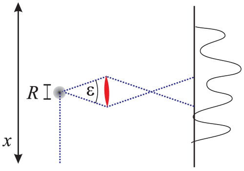
 -axis scatters off a probe within
an interaction region of radius
-axis scatters off a probe within
an interaction region of radius  and is detected by a microscope (indicated by a lens and screen)
with opening angle
and is detected by a microscope (indicated by a lens and screen)
with opening angle  .
. We know today that Heisenberg’s uncertainty is not just a peculiarity of a measurement method but
much more than that – it is a fundamental property of the quantum nature of matter. It does not, strictly
speaking, even make sense to consider the position and momentum of the particle at the same time.
Consequently, instead of speaking about the photon scattering off the particle as if that would happen in
one particular point, we should speak of the photon having a strong interaction with the particle in some
region of size  .
.
Now we will include gravity in the picture, following the treatment of Mead [222*]. For any interaction to
take place and subsequent measurement to be possible, the time elapsed between the interaction and
measurement has to be at least on the order of the time,  , the photon needs to travel the distance
  ,
so that
,
so that  . The photon carries an energy that, though in general tiny, exerts a gravitational pull on
the particle whose position we wish to measure. The gravitational acceleration acting on the particle is at
least on the order of
. The photon carries an energy that, though in general tiny, exerts a gravitational pull on
the particle whose position we wish to measure. The gravitational acceleration acting on the particle is at
least on the order of

 , or
Thus, in the time
, or
Thus, in the time 
 , the acquired velocity allows the particle to travel a distance of
However, since the direction of the photon was unknown to within the angle
, the acquired velocity allows the particle to travel a distance of
However, since the direction of the photon was unknown to within the angle 
 , the direction of the
acceleration and the motion of the particle is also unknown. Projection on the
, the direction of the
acceleration and the motion of the particle is also unknown. Projection on the  -axis then yields the
additional uncertainty of
Combining (8*) with (2*), one obtains
One can refine this argument by taking into account that strictly speaking during the measurement, the
momentum of the photon,
-axis then yields the
additional uncertainty of
Combining (8*) with (2*), one obtains
One can refine this argument by taking into account that strictly speaking during the measurement, the
momentum of the photon, 

 , increases by
  , where
  is the mass of the particle. This
increases the uncertainty in the particle’s momentum (3*) to
and, for the time the photon is in the interaction region, translates into a position uncertainty
is the mass of the particle. This
increases the uncertainty in the particle’s momentum (3*) to
and, for the time the photon is in the interaction region, translates into a position uncertainty

 which is larger than the previously found uncertainty (8*) and thus (9*) still follows.

Adler and Santiago [3*] offer pretty much the same argument, but add that the particle’s
momentum uncertainty  should be on the order of the photon’s momentum
  . Then one finds


These limitations, refinements of which we will discuss in the following Sections 3.1.2 – 3.1.7, apply to the possible spatial resolution in a microscope-like measurement. At the high energies necessary to reach the Planckian limit, the scattering is unlikely to be elastic, but the same considerations apply to inelastic scattering events. Heisenberg’s microscope revealed a fundamental limit that is a consequence of the non-commutativity of position and momentum operators in quantum mechanics. The question that the GUP then raises is what modification of quantum mechanics would give rise to the generalized uncertainty, a question we will return to in Section 4.2.
Another related argument has been put forward by Scardigli [275], who employs the idea that once one arrives at energies of about the Planck mass and concentrates them to within a volume of radius of the Planck length, one creates tiny black holes, which subsequently evaporate. This effects scales in the same way as the one discussed here, and one arrives again at (13*).
3.1.2 The general relativistic Heisenberg microscope
The above result makes use of Newtonian gravity, and has to be refined when one takes into account general
relativity. Before we look into the details, let us start with a heuristic but instructive argument. One of the
most general features of general relativity is the formation of black holes under certain circumstances,
roughly speaking when the energy density in some region of spacetime becomes too high. Once matter
becomes very dense, its gravitational pull leads to a total collapse that ends in the formation of a
horizon.8
It is usually assumed that the Hoop conjecture holds [306]: If an amount of energy  is compacted at any
time into a region whose circumference in every direction is
is compacted at any
time into a region whose circumference in every direction is  , then the region will eventually
develop into a black hole. The Hoop conjecture is unproven, but we know from both analytical and
numerical studies that it holds to very good precision [107, 168].
, then the region will eventually
develop into a black hole. The Hoop conjecture is unproven, but we know from both analytical and
numerical studies that it holds to very good precision [107, 168].
Consider now that we have a particle of energy  . Its extension
  has to be larger than the
Compton wavelength associated to the energy, so
has to be larger than the
Compton wavelength associated to the energy, so  . Thus, the larger the energy, the better the
particle can be focused. On the other hand, if the extension drops below
. Thus, the larger the energy, the better the
particle can be focused. On the other hand, if the extension drops below  , then a black hole is
formed with radius
, then a black hole is
formed with radius  . The important point to notice here is that the extension of the black hole grows
linearly with the energy, and therefore one can achieve a minimal possible extension, which is on the order
of
. The important point to notice here is that the extension of the black hole grows
linearly with the energy, and therefore one can achieve a minimal possible extension, which is on the order
of  .
.
For the more detailed argument, we follow Mead [222*] with the general relativistic version of the
Heisenberg microscope that was discussed in Section 3.1.1. Again, we have a particle whose position we
want to measure by help of a test particle. The test particle has a momentum vector  , and for
completeness we consider a particle with rest mass
, and for
completeness we consider a particle with rest mass  , though we will see later that the tightest
constraints come from the limit
, though we will see later that the tightest
constraints come from the limit  .
.
The velocity  of the test particle is
 , and
, and  . As before, the test particle moves in the
  direction. The task is
now to compute the gravitational field of the test particle and the motion it causes on the measured
particle.
direction. The task is
now to compute the gravitational field of the test particle and the motion it causes on the measured
particle.
To obtain the metric that the test particle creates, we first change into the rest frame of the particle by
boosting into  -direction. Denoting the new coordinates with primes, the measured particle moves
towards the test particle in direction
-direction. Denoting the new coordinates with primes, the measured particle moves
towards the test particle in direction  , and the metric is a Schwarzschild metric. We will only need it
on the
, and the metric is a Schwarzschild metric. We will only need it
on the  -axis where we have
  , and thus


 , and the same for the primed coordinates, the Lorentz
boost from the primed to unprimed coordinates yields in the rest frame of the measured particle
where
Here,
, and the same for the primed coordinates, the Lorentz
boost from the primed to unprimed coordinates yields in the rest frame of the measured particle
where
Here, 

 is the mean distance between the test particle and the measured particle. To avoid a
horizon in the rest frame, we must have
is the mean distance between the test particle and the measured particle. To avoid a
horizon in the rest frame, we must have  , and thus from Eq. (21*)
Because of Eq. (2*),
, and thus from Eq. (21*)
Because of Eq. (2*), 
 but also
  , which is the area in which the particle may scatter,
thus
We see from this that, as long as
, which is the area in which the particle may scatter,
thus
We see from this that, as long as 
 , the previously found lower bound on the spatial resolution
 can already be read off here, and we turn our attention towards the case where
  . From
(21*) we see that this means we work in the limit where
. From
(21*) we see that this means we work in the limit where  .
.
To proceed, we need to estimate now how much the measured particle moves due to the test particle’s
vicinity. For this, we note that the world line of the measured particle must be timelike. We denote the
velocity in the  -direction with
  , then we need


 . We simplify the requirement of Eq. (24*) by leaving
  alone on the left
side of the inequality, subtracting
alone on the left
side of the inequality, subtracting  and dividing by
  . Taking into account that
  and
and
 , one finds after some algebra
and
One arrives at this estimate with reduced effort if one makes it clear to oneself what we want to estimate.
We want to know, as previously, how much the particle, whose position we are trying to measure, will move
due to the gravitational attraction of the particle we are using for the measurement. The faster the particles
pass by each other, the shorter the interaction time and, all other things being equal, the less the particle
we want to measure will move. Thus, if we consider a photon with
, one finds after some algebra
and
One arrives at this estimate with reduced effort if one makes it clear to oneself what we want to estimate.
We want to know, as previously, how much the particle, whose position we are trying to measure, will move
due to the gravitational attraction of the particle we are using for the measurement. The faster the particles
pass by each other, the shorter the interaction time and, all other things being equal, the less the particle
we want to measure will move. Thus, if we consider a photon with 

 , we are dealing with
the case with the least influence, and if we find a minimal length in this case, it should be
there for all cases. Setting
, we are dealing with
the case with the least influence, and if we find a minimal length in this case, it should be
there for all cases. Setting  , one obtains the inequality Eq. (27*) with greatly reduced
work.
, one obtains the inequality Eq. (27*) with greatly reduced
work.
Now we can continue as before in the non-relativistic case. The time  required for the test particle to
move a distance
required for the test particle to
move a distance  away from the measured particle is at least
  , and during this time the
measured particle moves a distance
, and during this time the
measured particle moves a distance

 , this means
and projection on the
, this means
and projection on the 
 -axis yields as before (compare to Eq. (8*)) for the uncertainty added to the
measured particle because the photon’s direction was known only to precision
-axis yields as before (compare to Eq. (8*)) for the uncertainty added to the
measured particle because the photon’s direction was known only to precision  This combines with (2*), to again give


Adler and Santiago [3*] found the same result by using the linear approximation of Einstein’s field
equation for a cylindrical source with length  and radius
  of comparable size, filled by a radiation field
with total energy
of comparable size, filled by a radiation field
with total energy  , and moving in the
  direction. With cylindrical coordinates
  , the line
element takes the form [3]
, the line
element takes the form [3]

 is given by
In this background, one can then compute the motion of the measured particle by using the Newtonian
limit of the geodesic equation, provided the particle remains non-relativistic. In the longitudinal direction,
along the motion of the test particle one finds
The derivative of
is given by
In this background, one can then compute the motion of the measured particle by using the Newtonian
limit of the geodesic equation, provided the particle remains non-relativistic. In the longitudinal direction,
along the motion of the test particle one finds
The derivative of 

 gives two delta-functions at the front and back of the cylinder with equal
momentum transfer but of opposite direction. The change in velocity to the measured particle is
Near the cylinder
gives two delta-functions at the front and back of the cylinder with equal
momentum transfer but of opposite direction. The change in velocity to the measured particle is
Near the cylinder 
 is of order one, and in the time of passage
  , the particle thus moves
approximately
which is, up to a factor of 2, the same result as Mead’s (29*). We note that Adler and Santiago’s argument
does not make use of the requirement that no black hole should be formed, but that the appropriateness of
the non-relativistic and weak-field limit is questionable.
, the particle thus moves
approximately
which is, up to a factor of 2, the same result as Mead’s (29*). We note that Adler and Santiago’s argument
does not make use of the requirement that no black hole should be formed, but that the appropriateness of
the non-relativistic and weak-field limit is questionable.

3.1.3 Limit to distance measurements
Wigner and Salecker [274] proposed the following thought experiment to show that the precision of length
measurements is limited. Consider that we try to measure a length by help of a clock that detects photons,
which are reflected by a mirror at distance  and return to the clock. Knowing the speed of light is
universal, from the travel-time of the photon we can then extract the distance it has traveled. How precisely
can we measure the distance in this way?
and return to the clock. Knowing the speed of light is
universal, from the travel-time of the photon we can then extract the distance it has traveled. How precisely
can we measure the distance in this way?
Consider that at emission of the photon, we know the position of the (non-relativistic) clock to precision
 . This means, according to the Heisenberg uncertainty principle, we cannot know its velocity to better
than
. This means, according to the Heisenberg uncertainty principle, we cannot know its velocity to better
than

 is the mass of the clock. During the time
  that the photon needed to travel towards
the mirror and back, the clock moves by
that the photon needed to travel towards
the mirror and back, the clock moves by  , and so acquires an uncertainty in position of
which bounds the accuracy by which we can determine the distance
, and so acquires an uncertainty in position of
which bounds the accuracy by which we can determine the distance 
 . The minimal value that this
uncertainty can take is found by varying with respect to
. The minimal value that this
uncertainty can take is found by varying with respect to  and reads
Taking into account that our measurement will not be causally connected to the rest of the world if it
creates a black hole, we require
and reads
Taking into account that our measurement will not be causally connected to the rest of the world if it
creates a black hole, we require 
 and thus

3.1.4 Limit to clock synchronization
From Mead’s [222*] investigation of the limit for the precision of distance measurements due to the gravitational force also follows a limit on the precision by which clocks can be synchronized.
We will consider the clock synchronization to be performed by the passing of light signals from some
standard clock to the clock under question. Since the emission of a photon with energy spread  by the
usual Heisenberg uncertainty is uncertain by
by the
usual Heisenberg uncertainty is uncertain by  , we have to take into account the same
uncertainty for the synchronization.
, we have to take into account the same
uncertainty for the synchronization.
The new ingredient comes again from the gravitational field of the photon, which interacts with the
clock in a region  over a time
  . If the clock (or the part of the clock that interacts with the
photon) remains stationary, the (proper) time it records stands in relation to
. If the clock (or the part of the clock that interacts with the
photon) remains stationary, the (proper) time it records stands in relation to  by
by  with
with
 in the rest frame of the clock, given by Eq. (20*), thus

Since the metric depends on the energy of the photon and this energy is not known precisely, the error
on  propagates into
  by
by

 , we can estimate
Multiplication of (45*) with the normal uncertainty
, we can estimate
Multiplication of (45*) with the normal uncertainty 
 yields
So we see that the precision by which clocks can be synchronized is also bound by the Planck
scale.
yields
So we see that the precision by which clocks can be synchronized is also bound by the Planck
scale.

However, strictly speaking the clock does not remain stationary during the interaction, since it moves
towards the photon due to the particles’ mutual gravitational attraction. If the clock has a velocity  ,
then the proper time it records is more generally given by
,
then the proper time it records is more generally given by

 and
and  and so with
 Therefore, taking into account that the clock does not remain stationary, one still arrives at
(46*).
Therefore, taking into account that the clock does not remain stationary, one still arrives at
(46*).

3.1.5 Limit to the measurement of the black-hole–horizon area
The above microscope experiment investigates how precisely one can measure the location of a
particle, and finds the precision bounded by the inevitable formation of a black hole. However,
this position uncertainty is for the location of the measured particle however and not for the
size of the black hole or its radius. There is a simple argument why one would expect there to
also be a limit to the precision by which the size of a black hole can be measured, first put
forward in [91]. When the mass of a black-hole approaches the Planck mass, the horizon radius
 associated to the mass becomes comparable to its Compton wavelength
  .
Then, quantum fluctuations in the position of the black hole should affect the definition of the
horizon.
.
Then, quantum fluctuations in the position of the black hole should affect the definition of the
horizon.
A somewhat more elaborate argument has been studied by Maggiore [208] by a thought experiment that makes use once again of Heisenberg’s microscope. However, this time one wants to measure not the position of a particle, but the area of a (non-rotating) charged black hole’s horizon. In Boyer–Lindquist coordinates, the horizon is located at the radius
where![[ ( 2 ) 12] RH = GM 1 + 1 − --Q--- , (50 ) GM 2](article192x.gif)
 is the charge and
  is the mass of the black hole.
To deduce the area of the black hole, we detect the black hole’s Hawking radiation and aim at tracing it
back to the emission point with the best possible accuracy. For the case of an extremal black hole
( ) the temperature is zero and we perturb the black hole by sending in photons from
asymptotic infinity and wait for re-emission.
) the temperature is zero and we perturb the black hole by sending in photons from
asymptotic infinity and wait for re-emission.
If the microscope detects a photon of some frequency  , it is subject to the usual uncertainty (2*)
arising from the photon’s finite wavelength that limits our knowledge about the photon’s origin. However, in
addition, during the process of emission the mass of the black hole changes from
, it is subject to the usual uncertainty (2*)
arising from the photon’s finite wavelength that limits our knowledge about the photon’s origin. However, in
addition, during the process of emission the mass of the black hole changes from  to
to  , and the
horizon radius, which we want to measure, has to change accordingly. If the energy of the photon is known
only up to an uncertainty
, and the
horizon radius, which we want to measure, has to change accordingly. If the energy of the photon is known
only up to an uncertainty  , then the error propagates into the precision by which we can deduce the
radius of the black hole
, then the error propagates into the precision by which we can deduce the
radius of the black hole

 one always finds
that
In an argument similar to that of Adler and Santiago discussed in Section 3.1.2, Maggiore then suggests
that the two uncertainties, the usual one inversely proportional to the photon’s energy and the additional
one (52*), should be linearly added to
where the constant
one always finds
that
In an argument similar to that of Adler and Santiago discussed in Section 3.1.2, Maggiore then suggests
that the two uncertainties, the usual one inversely proportional to the photon’s energy and the additional
one (52*), should be linearly added to
where the constant 

 would have to be fixed by using a specific theory. Minimizing the possible position
uncertainty, one thus finds again a minimum error of
would have to be fixed by using a specific theory. Minimizing the possible position
uncertainty, one thus finds again a minimum error of  .
.
It is clear that the uncertainty Maggiore considered is of a different kind than the one considered by Mead, though both have the same origin. Maggiore’s uncertainty is due to the impossibility of directly measuring a black hole without it emitting a particle that carries energy and thereby changing the black-hole–horizon area. The smaller the wavelength of the emitted particle, the larger the so-caused distortion. Mead’s uncertainty is due to the formation of black holes if one uses probes of too high an energy, which limits the possible precision. But both uncertainties go back to the relation between a black hole’s area and its mass.
3.1.6 A device-independent limit for non-relativistic particles
Even though the Heisenberg microscope is a very general instrument and the above considerations carry over to many other experiments, one may wonder if there is not some possibility to overcome the limitation of the Planck length by use of massive test particles that have smaller Compton wavelengths, or interferometers that allow one to improve on the limitations on measurement precisions set by the test particles’ wavelengths. To fill in this gap, Calmet, Graesser and Hsu [72, 73] put forward an elegant device-independent argument. They first consider a discrete spacetime with a sub-Planckian spacing and then show that no experiment is able to rule out this possibility. The point of the argument is not the particular spacetime discreteness they consider, but that it cannot be ruled out in principle.
The setting is a position operator  with discrete eigenvalues
  that have a separation of order
 or smaller. To exclude the model, one would have to measure position eigenvalues
  and
and  , for
example, of some test particle of mass
, for
example, of some test particle of mass  , with
  . Assuming the non-relativistic
Schrödinger equation without potential, the time-evolution of the position operator is given by
. Assuming the non-relativistic
Schrödinger equation without potential, the time-evolution of the position operator is given by
![dxˆ(t)∕dt = i[ ˆH, ˆx(t)] = pˆ∕M](article213x.gif) , and thus
, and thus

![1 ΔA ΔB ≥ --⟨[ ˆA,Bˆ]⟩, (55 ) 2i](article215x.gif)
 denotes, as usual, the variance and
  the expectation value of the operator. From (54*) one
has
and thus
Since one needs to measure two positions to determine a distance, the minimal uncertainty to the distance
measurement is
the expectation value of the operator. From (54*) one
has
and thus
Since one needs to measure two positions to determine a distance, the minimal uncertainty to the distance
measurement is
![-t- [ˆx(0), ˆx(t)] = iM , (56 )](article218x.gif)

This is the same bound as previously discussed in Section 3.1.3 for the measurement of distances by help of a clock, yet we arrived here at this bound without making assumptions about exactly what is measured and how. If we take into account gravity, the argument can be completed similar to Wigner’s and still without making assumptions about the type of measurement, as follows.
We use an apparatus of size  . To get the spacing as precise as possible, we would use a test particle
of high mass. But then we will run into the, by now familiar, problem of black-hole formation when the
mass becomes too large, so we have to require
. To get the spacing as precise as possible, we would use a test particle
of high mass. But then we will run into the, by now familiar, problem of black-hole formation when the
mass becomes too large, so we have to require

 . Taken together, one finds
and thus once again the possible precision of a position measurement is limited by the Planck
length.
. Taken together, one finds
and thus once again the possible precision of a position measurement is limited by the Planck
length.

A similar argument was made by Ng and van Dam [238], who also pointed out that with this thought experiment one can obtain a scaling for the uncertainty with the third root of the size of the detector. If one adds the position uncertainty (58*) from the non-vanishing commutator to the gravitational one, one finds
Optimizing this expression with respect to the mass that yields a minimal uncertainty, one finds
 (up to factors of order one) and, inserting this value of
  in (61*), thus
Since
in (61*), thus
Since 
 too should be larger than the Planck scale this is, of course, consistent with the previously-found
minimal uncertainty.
too should be larger than the Planck scale this is, of course, consistent with the previously-found
minimal uncertainty.
Ng and van Dam further argue that this uncertainty induces a minimum error in measurements of
energy and momenta. By noting that the uncertainty  of a length
  is indistinguishable from an
uncertainty of the metric components used to measure the length,
is indistinguishable from an
uncertainty of the metric components used to measure the length,  , the inequality (62*) leads
to
, the inequality (62*) leads
to
 , so this uncertainty for the metric
further induces an uncertainty for the entries of
, so this uncertainty for the metric
further induces an uncertainty for the entries of  Consider now using a test particle of momentum
 to probe the physics at scale
  , thus
  .
Then its uncertainty would be on the order of
.
Then its uncertainty would be on the order of

However, note that the scaling found by Ng and van Dam only follows if one works with the masses that minimize the uncertainty (61*). Then, even if one uses a detector of the approximate extension of a cm, the corresponding mass of the ‘particle’ we have to work with would be about a ton. With such a mass one has to worry about very different uncertainties. For particles with masses below the Planck mass on the other hand, the size of the detector would have to be below the Planck length, which makes no sense since its extension too has to be subject to the minimal position uncertainty.
3.1.7 Limits on the measurement of spacetime volumes
The observant reader will have noticed that almost all of the above estimates have explicitly or implicitly made use of spherical symmetry. The one exception is the argument by Adler and Santiago in Section 3.1.2 that employed cylindrical symmetry. However, it was also assumed there that the length and the radius of the cylinder are of comparable size.
In the general case, when the dimensions of the test particle in different directions are very unequal, the Hoop conjecture does not forbid any one direction to be smaller than the Schwarzschild radius to prevent collapse of some matter distribution, as long as at least one other direction is larger than the Schwarzschild radius. The question then arises what limits that rely on black-hole formation can still be derived in the general case.
A heuristic motivation of the following argument can be found in [101*], but here we will follow the more
detailed argument by Tomassini and Viaggiu [307]. In the absence of spherical symmetry, one may still use
Penrose’s isoperimetric-type conjecture, according to which the apparent horizon is always smaller than or
equal to the event horizon, which in turn is smaller than or equal to  , where
  is as before the
energy of the test particle.
is as before the
energy of the test particle.
Then, without spherical symmetry the requirement that no black hole ruins our ability to resolve short
distances is weakened from the energy distribution having a radius larger than the Schwarzschild radius, to
the requirement that the area  , which encloses
  is large enough to prevent Penrose’s condition for
horizon formation
is large enough to prevent Penrose’s condition for
horizon formation

 that, by the normal uncertainty principle, is larger than
 . Taking into account this uncertainty on the energy, one has

Now we have to make some assumption for the geometry of the object, which will inevitably be a
crude estimate. While an exact bound will depend on the shape of the matter distribution, we
will here just be interested in obtaining a bound that depends on the three different spatial
extensions, and is qualitatively correct. To that end, we assume the mass distribution fits into
some smallest box with side-lengths  , which is similar to the limiting area

 to take into account different possible geometries. A comparison with
the spherical case,
to take into account different possible geometries. A comparison with
the spherical case,  , fixes
  . With Eq. (67*) one obtains
Since
one also has
which confirms the limit obtained earlier by heuristic reasoning in [101].
. With Eq. (67*) one obtains
Since
one also has
which confirms the limit obtained earlier by heuristic reasoning in [101].


Thus, as anticipated, taking into account that a black hole must not necessarily form if the spatial
extension of a matter distribution is smaller than the Schwarzschild radius in only one direction, the
uncertainty we arrive at here depends on the extension in all three directions, rather than applying
separately to each of them. Here we have replaced  by the inverse of
  , rather than combining with
Eq. (2*), but this is just a matter of presentation.
, rather than combining with
Eq. (2*), but this is just a matter of presentation.
Since the bound on the volumes (71*) follows from the bounds on spatial and temporal intervals we found
above, the relevant question here is not whether ?? is fulfilled, but whether the bound  can be
violated [165].
can be
violated [165].
To address that question, note that the quantities  in the above argument by Tomassini and
Viaggiu differ from the ones we derived bounds for in Sections 3.1.1 – 3.1.6. Previously, the
in the above argument by Tomassini and
Viaggiu differ from the ones we derived bounds for in Sections 3.1.1 – 3.1.6. Previously, the  was the
precision by which one can measure the position of a particle with help of the test particle. Here, the
was the
precision by which one can measure the position of a particle with help of the test particle. Here, the  are the smallest possible extensions of the test particle (in the rest frame), which with spherical symmetry
would just be the Schwarzschild radius. The step in which one studies the motion of the measured particle
that is induced by the gravitational field of the test particle is missing in this argument. Thus,
while the above estimate correctly points out the relevance of non-spherical symmetries, the
argument does not support the conclusion that it is possible to test spatial distances to arbitrary
precision.
are the smallest possible extensions of the test particle (in the rest frame), which with spherical symmetry
would just be the Schwarzschild radius. The step in which one studies the motion of the measured particle
that is induced by the gravitational field of the test particle is missing in this argument. Thus,
while the above estimate correctly points out the relevance of non-spherical symmetries, the
argument does not support the conclusion that it is possible to test spatial distances to arbitrary
precision.
The main obstacle to completion of this argument is that in the context of quantum field theory we are eventually dealing with particles probing particles. To avoid spherical symmetry, we would need different objects as probes, which would require more information about the fundamental nature of matter. We will come back to this point in Section 3.2.3.
3.2 String theory
String theory is one of the leading candidates for a theory of quantum gravity. Many textbooks
have been dedicated to the topic, and the interested reader can also find excellent resources
online [187, 278, 235, 299]. For the following we will not need many details. Most importantly, we need to
know that a string is described by a 2-dimensional surface swept out in a higher-dimensional spacetime. The
total number of spatial dimensions that supersymmetric string theory requires for consistency is nine, i.e.,
there are six spatial dimensions in addition to the three we are used to. In the following we will denote the
total number of dimensions, both time and space-like, with  . In this Subsection, Greek indices run from
 to
to  .
.
The two-dimensional surface swept out by the string in the  -dimensional spacetime is referred to as
the ‘worldsheet,’ will be denoted by
-dimensional spacetime is referred to as
the ‘worldsheet,’ will be denoted by  , and will be parameterized by (dimensionless) parameters
  and
and  , where
  is its time-like direction, and
  runs conventionally from 0 to
  . A
string has discrete excitations, and its state can be expanded in a series of these excitations
plus the motion of the center of mass. Due to conformal invariance, the worldsheet carries a
complex structure and thus becomes a Riemann surface, whose complex coordinates we will
denote with
. A
string has discrete excitations, and its state can be expanded in a series of these excitations
plus the motion of the center of mass. Due to conformal invariance, the worldsheet carries a
complex structure and thus becomes a Riemann surface, whose complex coordinates we will
denote with  and
and  . Scattering amplitudes in string theory are a sum over such surfaces.
In the following  is the string scale, and
  . The string scale is related to the Planck scale by
 , where
  is the string coupling constant. Contrary to what the name suggests, the string
coupling constant is not constant, but depends on the value of a scalar field known as the dilaton.
is the string coupling constant. Contrary to what the name suggests, the string
coupling constant is not constant, but depends on the value of a scalar field known as the dilaton.
To avoid conflict with observation, the additional spatial dimensions of string theory have to be
compactified. The compactification scale is usually thought to be about the Planck length, and far below
experimental accessibility. The possibility that the extensions of the extra dimensions (or at least some of
them) might be much larger than the Planck length and thus possibly experimentally accessible, has been
studied in models with a large compactification volume and lowered Planck scale, see, e.g., [1]. We will not
discuss these models here, but mention in passing that they demonstrate the possibility that the ‘true’
higher-dimensional Planck mass is in fact much smaller than  , and correspondingly the ‘true’
higher-dimensional Planck length, and with it the minimal length, much larger than
, and correspondingly the ‘true’
higher-dimensional Planck length, and with it the minimal length, much larger than  . That such
possibilities exist means, whether or not the model with extra dimensions are realized in nature, that we
should, in principle, consider the minimal length a free parameter that has to be constrained by
experiment.
. That such
possibilities exist means, whether or not the model with extra dimensions are realized in nature, that we
should, in principle, consider the minimal length a free parameter that has to be constrained by
experiment.
String theory is also one of the motivations to look into non-commutative geometries. Non-commutative geometry will be discussed separately in Section 3.6. A section on matrix models will be included in a future update.
3.2.1 Generalized uncertainty
The following argument, put forward by Susskind [297, 298], will provide us with an insightful examination
that illustrates how a string is different from a point particle and what consequences this difference has for
our ability to resolve structures at shortest distances. We consider a free string in light cone coordinates,
 with the parameterization
  , where
  is the momentum in the
direction
is the momentum in the
direction  and constant along the string. In the light-cone gauge, the string has no oscillations in the
 direction by construction.
The transverse dimensions are the remaining  with
with  . The normal mode decomposition of the
transverse coordinates has the form
. The normal mode decomposition of the
transverse coordinates has the form

 is the (transverse location of) the center of mass of the string. The coefficients
  and
and  are normalized to
 ![i j i j ij [αn,α m] = [&tidle;αn, &tidle;α m] = − im δ δm,− n](article292x.gif) , and
, and ![i j [α&tidle;n,αm ] = 0](article293x.gif) . Since
the components
. Since
the components  are real, the coefficients have to fulfill the relations
  and
and
 .
.
We can then estimate the transverse size  of the string by

 , which
corresponds to some resolution time
, which
corresponds to some resolution time  , allows us to cut off modes with frequency
 or mode number
  . Then, for large
  , the sum becomes approximately
Thus, the transverse extension of the string grows with the energy that the string is tested by, though only
very slowly so.
, the sum becomes approximately
Thus, the transverse extension of the string grows with the energy that the string is tested by, though only
very slowly so.

To determine the spread in the longitudinal direction  , one needs to know that in light-cone
coordinates the constraint equations on the string have the consequence that
, one needs to know that in light-cone
coordinates the constraint equations on the string have the consequence that  is related
to the transverse directions so that it is given in terms of the light-cone Virasoro generators
is related
to the transverse directions so that it is given in terms of the light-cone Virasoro generators

 and
and  fulfill the Virasoro algebra. Therefore, the longitudinal spread in the ground
state gains a factor
fulfill the Virasoro algebra. Therefore, the longitudinal spread in the ground
state gains a factor  over the transverse case, and diverges as
Again, this result has an unphysical divergence, that we deal with the same way as before by taking into
account a finite resolution
over the transverse case, and diverges as
Again, this result has an unphysical divergence, that we deal with the same way as before by taking into
account a finite resolution 
 , corresponding to the inverse of the energy by which the string is probed.
Then one finds for large
, corresponding to the inverse of the energy by which the string is probed.
Then one finds for large  approximately
Thus, this heuristic argument suggests that the longitudinal spread of the string grows linearly with the
energy at which it is probed.
approximately
Thus, this heuristic argument suggests that the longitudinal spread of the string grows linearly with the
energy at which it is probed.
The above heuristic argument is supported by many rigorous calculations. That string scattering leads
to a modification of the Heisenberg uncertainty relation has been shown in several studies of string
scattering at high energies performed in the late 1980s [140*, 310, 228*]. Gross and Mende [140] put forward
a now well-known analysis of the classic solution for the trajectories of a string worldsheet describing a
scattering event with external momenta  . In the lowest tree approximation they found for the extension
of the string
. In the lowest tree approximation they found for the extension
of the string

 are the positions of the vertex
operators on the Riemann surface corresponding to the asymptotic states with momenta
are the positions of the vertex
operators on the Riemann surface corresponding to the asymptotic states with momenta  . Thus, as
previously, the extension grows linearly with the energy. One also finds that the surface of the string grows
with
. Thus, as
previously, the extension grows linearly with the energy. One also finds that the surface of the string grows
with  , where
  is the genus of the expansion, and that the fixed angle scattering amplitude
at high energies falls exponentially with the square of the center-of-mass energy
is the genus of the expansion, and that the fixed angle scattering amplitude
at high energies falls exponentially with the square of the center-of-mass energy  (times
 ).
).
One can interpret this spread of the string in terms of a GUP by taking into account that at high energies the spread grows linearly with the energy. Together with the normal uncertainty, one obtains
again the GUP that gives rise to a minimally-possible spatial resolution.
However, the exponential fall-off of the tree amplitude depends on the genus of the expansion, and is
dominated by the large  contributions because these decrease slower. The Borel resummation of the
series has been calculated in [228] and it was found that the tree level approximation is valid only for an
intermediate range of energies, and for
contributions because these decrease slower. The Borel resummation of the
series has been calculated in [228] and it was found that the tree level approximation is valid only for an
intermediate range of energies, and for  the amplitude decreases much slower than
the tree-level result would lead one to expect. Yoneya [318*] has furthermore argued that this
behavior does not properly take into account non-perturbative effects, and thus the generalized
uncertainty should not be regarded as generally valid in string theory. We will discuss this in
Section 3.2.3.
the amplitude decreases much slower than
the tree-level result would lead one to expect. Yoneya [318*] has furthermore argued that this
behavior does not properly take into account non-perturbative effects, and thus the generalized
uncertainty should not be regarded as generally valid in string theory. We will discuss this in
Section 3.2.3.
It has been proposed that the resistance of the string to attempts to localize it plays a role in resolving the black-hole information-loss paradox [204]. In fact, one can wonder if the high energy behavior of the string acts against and eventually prevents the formation of black holes in elementary particle collisions. It has been suggested in [10, 9, 11] that string effects might become important at impact parameters far greater than those required to form black holes, opening up the possibility that black holes might not form.
The completely opposite point of view, that high energy scattering is ultimately entirely dominated by black-hole production, has also been put forward [48, 131*]. Giddings and Thomas found an indication of how gravity prevents probes of distance shorter than the Planck scale [131] and discussed the ‘the end of short-distance physics’; Banks aptly named it ‘asymptotic darkness’ [47]. A recent study of string scattering at high energies [127] found no evidence that the extendedness of the string interferes with black-hole formation. The subject of string scattering in the trans-Planckian regime is subject of ongoing research, see, e.g., [12, 90, 130] and references therein.
Let us also briefly mention that the spread of the string just discussed should not be confused with the length of the string. (For a schematic illustration see Figure 2*.) The length of a string in the transverse direction is
where the sum is taken in the transverse direction, and has been studied numerically in [173*]. In this study, it has been shown that when one increases the cut-off on the modes, the string becomes space-filling, and fills space densely (i.e., it comes arbitrarily close to any point in space).
3.2.2 Spacetime uncertainty
Yoneya [318*] argued that the GUP in string theory is not generally valid. To begin with, it is not clear whether the Borel resummation of the perturbative expansion leads to correct non-perturbative results. And, after the original works on the generalized uncertainty in string theory, it has become understood that string theory gives rise to higher-dimensional membranes that are dynamical objects in their own right. These higher-dimensional membranes significantly change the picture painted by high energy string scattering, as we will see in 3.2.3. However, even if the GUP is not generally valid, there might be a different uncertainty principle that string theory conforms to, that is a spacetime uncertainty of the form

This spacetime uncertainty has been motivated by Yoneya to arise from conformal symmetry [317*, 318*] as follows.
Suppose we are dealing with a Riemann surface with metric  that parameterizes the
string. In string theory, these surfaces appear in all path integrals and thus amplitudes, and they are thus of
central importance for all possible processes. Let us denote with
that parameterizes the
string. In string theory, these surfaces appear in all path integrals and thus amplitudes, and they are thus of
central importance for all possible processes. Let us denote with  a finite region in that surface, and
with
a finite region in that surface, and
with  the set of all curves in
  . The length of some curve
  is then
  .
However, this length that we are used to from differential geometry is not conformally invariant. To find a
length that captures only the physically-relevant information, one can use a distance measure known as the
‘extremal length’
.
However, this length that we are used to from differential geometry is not conformally invariant. To find a
length that captures only the physically-relevant information, one can use a distance measure known as the
‘extremal length’ 


 is a generic polygon with four sides and four corners, with pairs of opposite sides named
 and
and  . Any more complicated shape can be assembled from such polygons. Let
  be the set of all curves connecting
  with
with  and
and  the set of all curves connecting
 with
with  . The extremal lengths
  and
and  then fulfill property [317*, 318*]

Conformal invariance allows us to deform the polygon, so instead of a general four-sided polygon, we can
consider a rectangle in particular, where the Euclidean length of the sides  will be
named
will be
named  and that of sides
  will be named
  . With a Minkowski metric, one of
these directions would be timelike and one spacelike. Then the extremal lengths are [317, 318*]
. With a Minkowski metric, one of
these directions would be timelike and one spacelike. Then the extremal lengths are [317, 318*]

 ) with the action
(Equal indices are summed over). As before,
) with the action
(Equal indices are summed over). As before, 
 are the target space coordinates of the string worldsheet.
We now decompose the coordinate
are the target space coordinates of the string worldsheet.
We now decompose the coordinate  into its real and imaginary part
  , and
consider a rectangular piece of the surface with the boundary conditions
If one integrates over the rectangular region, the action contains a factor
, and
consider a rectangular piece of the surface with the boundary conditions
If one integrates over the rectangular region, the action contains a factor 
 and the
path integral thus contains a factor of the form
Thus, the width of these contributions is given by the extremal length times the string scale, which
quantifies the variance of
and the
path integral thus contains a factor of the form
Thus, the width of these contributions is given by the extremal length times the string scale, which
quantifies the variance of 
 and
and  by
In particular the product of both satisfies the condition
Thus, probing short distances along the spatial and temporal directions simultaneously is not
possible to arbitrary precision, lending support to the existence of a spacetime uncertainty of the
form (82*). Yoneya notes [318*] that this argument cannot in this simple fashion be carried over
to more complicated shapes. Thus, at present the spacetime uncertainty has the status of a
conjecture. However, the power of this argument rests in it only relying on conformal invariance,
which makes it plausible that, in contrast to the GUP, it is universally and non-perturbatively
valid.
by
In particular the product of both satisfies the condition
Thus, probing short distances along the spatial and temporal directions simultaneously is not
possible to arbitrary precision, lending support to the existence of a spacetime uncertainty of the
form (82*). Yoneya notes [318*] that this argument cannot in this simple fashion be carried over
to more complicated shapes. Thus, at present the spacetime uncertainty has the status of a
conjecture. However, the power of this argument rests in it only relying on conformal invariance,
which makes it plausible that, in contrast to the GUP, it is universally and non-perturbatively
valid.


3.2.3 Taking into account Dp-Branes
The endpoints of open strings obey boundary conditions, either of the Neumann type or of the Dirichlet type or a mixture of both. For Dirichlet boundary conditions, the submanifold on which open strings end is called a Dirichlet brane, or Dp-brane for short, where p is an integer denoting the dimension of the submanifold. A D0-brane is a point, sometimes called a D-particle; a D1-brane is a one-dimensional object, also called a D-string; and so on, all the way up to D9-branes.
These higher-dimensional objects that arise in string theory have a dynamics in their own right, and have given rise to a great many insights, especially with respect to dualities between different sectors of the theory, and the study of higher-dimensional black holes [170, 45*].
Dp-branes have a tension of  ; that is, in the weak coupling limit, they become very
rigid. Thus, one might suspect D-particles to show evidence for structure on distances at least down to
; that is, in the weak coupling limit, they become very
rigid. Thus, one might suspect D-particles to show evidence for structure on distances at least down to
 .
.
Taking into account the scattering of Dp-branes indeed changes the conclusions we could draw from the earlier-discussed thought experiments. We have seen that this was already the case for strings, but we can expect that Dp-branes change the picture even more dramatically. At high energies, strings can convert energy into potential energy, thereby increasing their extension and counteracting the attempt to probe small distances. Therefore, strings do not make good candidates to probe small structures, and to probe the structures of Dp-branes, one would best scatter them off each other. As Bachas put it [45*], the “small dynamical scale of D-particles cannot be seen by using fundamental-string probes – one cannot probe a needle with a jelly pudding, only with a second needle!”
That with Dp-branes new scaling behaviors enter the physics of shortest distances has been pointed out
by Shenker [283], and in particular the D-particle scattering has been studied in great detail by Douglas et
al. [103*]. It was shown there that indeed slow moving D-particles can probe distances below the
(ten-dimensional) Planck scale and even below the string scale. For these D-particles, it has been found that
structures exist down to  .
.
To get a feeling for the scales involved here, let us first reconsider the scaling arguments on black-hole
formation, now in a higher-dimensional spacetime. The Newtonian potential  of a higher-dimensional
point charge with energy
of a higher-dimensional
point charge with energy  , or the perturbation of
  , in
, in  dimensions, is qualitatively of
the form
dimensions, is qualitatively of
the form

 is the spatial extension, and
  is the
  -dimensional Newton’s constant,
related to the Planck length as
-dimensional Newton’s constant,
related to the Planck length as  . Thus, the horizon or the zero of
  is located at
With
is located at
With 
 , for some time by which we test the geometry, to prevent black-hole formation for
 , one thus has to require
re-expressed in terms of string coupling and tension. We see that in the weak coupling limit, this lower
bound can be small, in particular it can be much below the string scale.
, one thus has to require
re-expressed in terms of string coupling and tension. We see that in the weak coupling limit, this lower
bound can be small, in particular it can be much below the string scale.

This relation between spatial and temporal resolution can now be contrasted with the spacetime uncertainty (82*), that sets the limits below which the classical notion of spacetime ceases to make sense. Both of these limits are shown in Figure 3* for comparison. The curves meet at
If we were to push our limits along the bound set by the spacetime uncertainty (red, solid line), then the best possible spatial resolution we could reach lies at
 , beyond which black-hole production takes
over. Below the spacetime uncertainty limit, it would actually become meaningless to talk about black holes
that resemble any classical object.
, beyond which black-hole production takes
over. Below the spacetime uncertainty limit, it would actually become meaningless to talk about black holes
that resemble any classical object.
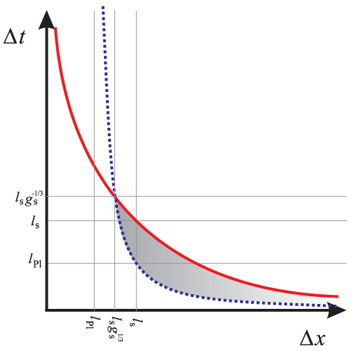
 dimensions, for
  (left) and
  (right). After [318*], Figure 1. Below the
bound from spacetime uncertainty yet above the black-hole bound that hides short-distance physics
(shaded region), the concept of classical geometry becomes meaningless.
(right). After [318*], Figure 1. Below the
bound from spacetime uncertainty yet above the black-hole bound that hides short-distance physics
(shaded region), the concept of classical geometry becomes meaningless. At first sight, this argument seems to suffer from the same problem as the previously examined
argument for volumes in Section 3.1.7. Rather than combining  with
with  to arrive at a weaker bound
than each alone would have to obey, one would have to show that in fact
to arrive at a weaker bound
than each alone would have to obey, one would have to show that in fact  can become arbitrarily
small. And, since the argument from black-hole collapse in 10 dimensions is essentially the same as Mead’s
in 4 dimensions, just with a different
can become arbitrarily
small. And, since the argument from black-hole collapse in 10 dimensions is essentially the same as Mead’s
in 4 dimensions, just with a different  -dependence of
  , if one would consider point particles in 10
dimensions, one finds along the same line of reasoning as in Section 3.1.2, that actually
, if one would consider point particles in 10
dimensions, one finds along the same line of reasoning as in Section 3.1.2, that actually  and
and
 .
.
However, here the situation is very different because fundamentally the objects we are dealing with are not particles but strings, and the interaction between Dp-branes is mediated by strings stretched between them. It is an inherently different behavior than what we can expect from the classical gravitational attraction between point particles. At low string coupling, the coupling of gravity is weak and in this limit then, the backreaction of the branes on the background becomes negligible. For these reasons, the D-particles distort each other less than point particles in a quantum field theory would, and this is what allows one to use them to probe very short distances.
The following estimate from [318] sheds light on the scales that we can test with D-particles in
particular. Suppose we use D-particles with velocity  and mass
  to probe a distance of
size
to probe a distance of
size  in time
  . Since
  , the uncertainty (94*) gives

But if the D-particle is slow, then its wavefunction behaves like that of a massive non-relativistic particle, so we have to take into account that the width spreads with time. For this, we can use the earlier-discussed bound Eq. (58*)
or If we add the uncertainties (96*) and (98*) and minimize the sum with respect to

 , we find that the spatial
uncertainty is minimal for
Thus, the total spatial uncertainty is bounded by
and with this one also has
which are the scales that we already identified in (95*) to be those of the best possible resolution compatible
with the spacetime uncertainty. Thus, we see that the D-particles saturate the spacetime uncertainty bound
and they can be used to test these short distances.
, we find that the spatial
uncertainty is minimal for
Thus, the total spatial uncertainty is bounded by
and with this one also has
which are the scales that we already identified in (95*) to be those of the best possible resolution compatible
with the spacetime uncertainty. Thus, we see that the D-particles saturate the spacetime uncertainty bound
and they can be used to test these short distances.


D-particle scattering has been studied in [103*] by use of a quantum mechanical toy model in which the
two particles are interacting by (unexcited) open strings stretched between them. The open strings create a
linear potential between the branes. At moderate velocities, repeated collisions can take place, since the
probability for all the open strings to annihilate between one collision and the next is small. At  ,
the time between collisions is on the order of
,
the time between collisions is on the order of  , corresponding to a resonance of width
 . By considering the conversion of kinetic energy into the potential of the strings, one sees that
the particles reach a maximal separation of
. By considering the conversion of kinetic energy into the potential of the strings, one sees that
the particles reach a maximal separation of  , realizing a test of the scales found
above.
, realizing a test of the scales found
above.
Douglas et al. [103*] offered a useful analogy of the involved scales to atomic physics; see Table (1). The
electron in a hydrogen atom moves with velocity determined by the fine-structure constant  , from which
it follows the characteristic size of the atom. For the D-particles, this corresponds to the maximal separation
in the repeated collisions. The analogy may be carried further than that in that higher-order corrections
should lead to energy shifts.
, from which
it follows the characteristic size of the atom. For the D-particles, this corresponds to the maximal separation
in the repeated collisions. The analogy may be carried further than that in that higher-order corrections
should lead to energy shifts.
| Electron | D-particle |
mass  |
mass  |
Compton wavelength  |
Compton wavelength  |
velocity  |
velocity  |
Bohr radius  |
size of resonance  |
energy levels  |
resonance energy  |
fine structure  |
energy shifts  |
The possibility to resolve such short distances with D-branes have been studied in many more
calculations; for a summary, see, for example, [45] and references therein. For our purposes, this estimate of
scales will be sufficient. We take away that D-branes, should they exist, would allow us to probe distances
down to  .
.
3.2.4 T-duality
In the presence of compactified spacelike dimensions, a string can acquire an entirely new property: It can
wrap around the compactified dimension. The number of times it wraps around, labeled by the integer  ,
is called the ‘winding-number.’ For simplicity, let us consider only one additional dimension, compactified
on a radius
,
is called the ‘winding-number.’ For simplicity, let us consider only one additional dimension, compactified
on a radius  . Then, in the direction of this coordinate, the string has to obey the boundary condition

The momentum in the direction of the additional coordinate is quantized in multiples of  , so the
expansion (compare to Eq. (72*)) reads
, so the
expansion (compare to Eq. (72*)) reads

 is some initial value. The momentum
  is then

The total energy of the quantized string with excitation  and winding number
  is formally
divergent, due to the contribution of all the oscillator’s zero point energies, and has to be renormalized.
After renormalization, the energy is
is formally
divergent, due to the contribution of all the oscillator’s zero point energies, and has to be renormalized.
After renormalization, the energy is
 runs over the non-compactified coordinates, and
  and
and  are the levels of excitations of the
left and right moving modes. Level matching requires
are the levels of excitations of the
left and right moving modes. Level matching requires  . In addition to the normal
contribution from the linear momentum, the string energy thus has a geometrically-quantized contribution
from the momentum into the extra dimension(s), labeled with
. In addition to the normal
contribution from the linear momentum, the string energy thus has a geometrically-quantized contribution
from the momentum into the extra dimension(s), labeled with  , an energy from the winding (more
winding stretches the string and thus needs energy), labeled with
, an energy from the winding (more
winding stretches the string and thus needs energy), labeled with  , and a renormalized contribution
from the Casimir energy. The important thing to note here is that this expression is invariant under the
exchange
i.e., an exchange of winding modes with excitations leaves mass spectrum invariant.
, and a renormalized contribution
from the Casimir energy. The important thing to note here is that this expression is invariant under the
exchange
i.e., an exchange of winding modes with excitations leaves mass spectrum invariant.

This symmetry is known as target-space duality, or T-duality for short. It carries over to
multiples extra dimensions, and can be shown to hold not only for the free string but also
during interactions. This means that for the string a distance below the string scale  is
meaningless because it corresponds to a distance larger than that; pictorially, a string that is highly
excited also has enough energy to stretch and wrap around the extra dimension. We have seen
in Section 3.2.3 that Dp-branes overcome limitations of string scattering, but T-duality is a
simple yet powerful way to understand why the ability of strings to resolves short distances is
limited.
is
meaningless because it corresponds to a distance larger than that; pictorially, a string that is highly
excited also has enough energy to stretch and wrap around the extra dimension. We have seen
in Section 3.2.3 that Dp-branes overcome limitations of string scattering, but T-duality is a
simple yet powerful way to understand why the ability of strings to resolves short distances is
limited.
This characteristic property of string theory has motivated a model that incorporates T-duality and compact extra dimensions into an effective path integral approach for a particle-like object that is described by the center-of-mass of the string, yet with a modified Green’s function, suggested in [285*, 111*, 291*].
In this approach it is assumed that the elementary constituents of matter are fundamentally strings that
propagate in a higher dimensional spacetime with compactified additional dimensions, so that the strings
can have excitations and winding numbers. By taking into account the excitations and winding
numbers, Fontanini et al. [285*, 111, 291] derive a modified Green’s function for a scalar field. In
the resulting double sum over  and
and  , the contribution from the
  and
and  zero modes is dropped. Note that this discards all massless modes as one sees from Eq. (106*).
As a result, the Green’s function obtained in this way no longer has the usual contribution
zero modes is dropped. Note that this discards all massless modes as one sees from Eq. (106*).
As a result, the Green’s function obtained in this way no longer has the usual contribution


 and
and  . Here,
  is the
modified Bessel function of the first kind, and
is the
modified Bessel function of the first kind, and  is the compactification scale of the extra
dimensions. For
is the compactification scale of the extra
dimensions. For  and
and  , in the limit where
  and the argument of
 is large compared to 1,
  , the modified Bessel function can be approximated by
and, in that limit, the term in the sum (109*) of the Green’s function takes the form
Thus, each term of the modified Green’s function falls off exponentially if the energies are large enough. The
Fourier transform of this limit of the momentum space propagator is
and one thus finds that the spacetime distance in the propagator acquires a finite correction term, which
one can interpret as a ‘zero point length’, at least in the Euclidean case.
, the modified Bessel function can be approximated by
and, in that limit, the term in the sum (109*) of the Green’s function takes the form
Thus, each term of the modified Green’s function falls off exponentially if the energies are large enough. The
Fourier transform of this limit of the momentum space propagator is
and one thus finds that the spacetime distance in the propagator acquires a finite correction term, which
one can interpret as a ‘zero point length’, at least in the Euclidean case.


It has been argued in [285] that this “captures the leading order correction from string theory”. This claim has not been supported by independent studies. However, this argument has been used as one of the motivations for the model with path integral duality that we will discuss in Section 4.7. The interesting thing to note here is that the minimal length that appears in this model is not determined by the Planck length, but by the radius of the compactified dimensions. It is worth emphasizing that this approach is manifestly Lorentz invariant.
3.3 Loop Quantum Gravity and Loop Quantum Cosmology
Loop Quantum Gravity (LQG) is a quantization of gravity by help of carefully constructed suitable variables for quantization, variables that have become known as the Ashtekar variables [39]. While LQG theory still lacks experimental confirmation, during the last two decades it has blossomed into an established research area. Here we will only roughly sketch the main idea to see how it entails a minimal length scale. For technical details, the interested reader is referred to the more specialized reviews [42, 304, 305, 229, 118*].
Since one wants to work with the Hamiltonian framework, one begins with the familiar 3+1 split of
spacetime. That is, one assumes that spacetime has topology  , i.e., it can be sliced into a set of
spacelike 3-dimensional hypersurfaces. Then, the metric can be parameterized with the lapse-function
, i.e., it can be sliced into a set of
spacelike 3-dimensional hypersurfaces. Then, the metric can be parameterized with the lapse-function  and the shift vector

 is the three metric on the slice. The three metric by itself does not suffice to completely describe
the four dimensional spacetime. If one wants to stick with quantities that make sense on the three
dimensional surfaces, in order to prepare for quantization, one needs in addition the ‘extrinsic curvature’
that describes how the metric changes along the slicing
where
is the three metric on the slice. The three metric by itself does not suffice to completely describe
the four dimensional spacetime. If one wants to stick with quantities that make sense on the three
dimensional surfaces, in order to prepare for quantization, one needs in addition the ‘extrinsic curvature’
that describes how the metric changes along the slicing
where 
 is the covariant three-derivative on the slice. So far, one is used to that from general
relativity.
is the covariant three-derivative on the slice. So far, one is used to that from general
relativity.
Next we introduce the triad or dreibein,  , which is a set of three vector fields

 (small, Latin, from the beginning of the alphabet) to a
locally-flat metric with indices
(small, Latin, from the beginning of the alphabet) to a
locally-flat metric with indices  (small, Latin, from the middle of the alphabet). The densitized triad
is the first set of variables used for quantization. The other set of variables is an
(small, Latin, from the middle of the alphabet). The densitized triad
is the first set of variables used for quantization. The other set of variables is an 
 connection
  ,
which is related to the connection on the manifold and the external curvature by
where the
,
which is related to the connection on the manifold and the external curvature by
where the 
 is the internal index and
  is the spin-connection. The dimensionless constant
 is the ‘Barbero–Immirzi parameter’. Its value can be fixed by requiring the black-hole entropy to match
with the semi-classical case, and comes out to be of order one.
is the ‘Barbero–Immirzi parameter’. Its value can be fixed by requiring the black-hole entropy to match
with the semi-classical case, and comes out to be of order one.
From the triads one can reconstruct the internal metric, and from  and the triad, one can
reconstruct the extrinsic curvature and thus one has a full description of spacetime. The reason for this
somewhat cumbersome reformulation of general relativity is that these variables do not only
recast gravity as a gauge theory, but are also canonically conjugated in the classical theory
and the triad, one can
reconstruct the extrinsic curvature and thus one has a full description of spacetime. The reason for this
somewhat cumbersome reformulation of general relativity is that these variables do not only
recast gravity as a gauge theory, but are also canonically conjugated in the classical theory

 and
and  to operators
  and
and  and replaces the Poisson bracket with commutators,
The Lagrangian of general relativity can then be rewritten in terms of the new variables, and the constraint
equations can be derived.
and replaces the Poisson bracket with commutators,
The Lagrangian of general relativity can then be rewritten in terms of the new variables, and the constraint
equations can be derived.
![[ ˆj ˆ&tidle;a ] b i 3 Ab(x),E i (y) = iβδaδjδ (x − y). (119 )](article489x.gif)
In the so-quantized theory one can then work with different representations, like one works in quantum
mechanics with the coordinate or momentum representation, just more complicated. One such
representation is the loop representation, an expansion of a state in a basis of (traces of) holonomies around
all possible closed loops. However, this basis is overcomplete. A more suitable basis are spin
networks  . Each such spin network is a graph with vertices and edges that carry labels of the
respective
. Each such spin network is a graph with vertices and edges that carry labels of the
respective  representation. In this basis, the states of LQG are then closed graphs, the
edges of which are labeled by irreducible
representation. In this basis, the states of LQG are then closed graphs, the
edges of which are labeled by irreducible  representations and the vertices by
  intertwiners.
The details of this approach to quantum gravity are far outside the scope of this review; for our purposes
we will just note that with this quantization scheme, one can construct operators for areas and volumes,
and with the expansion in the spin-network basis  , one can calculate the eigenvalues of these operators,
roughly as follows.
, one can calculate the eigenvalues of these operators,
roughly as follows.
Given a two-surface  that is parameterized by two coordinates
  with the third coordinate
 on the surface, the area of the surface is

 is the metric determinant on the surface. In terms of the triad, this can be
written as
This area can be promoted to an operator, essentially by making the triads operators, though to deal with
the square root of a product of these operators one has to average the operators over smearing
functions and take the limit of these smearing functions to delta functions. One can then act
with the so-constructed operator on the states of the spin network and obtain the eigenvalues
where the sum is taken over all edges of the network that pierce the surface
is the metric determinant on the surface. In terms of the triad, this can be
written as
This area can be promoted to an operator, essentially by making the triads operators, though to deal with
the square root of a product of these operators one has to average the operators over smearing
functions and take the limit of these smearing functions to delta functions. One can then act
with the so-constructed operator on the states of the spin network and obtain the eigenvalues
where the sum is taken over all edges of the network that pierce the surface 

 , and
, and  , a positive
half-integer, are the representation labels on the edge. This way, one finds that LQG has a minimum area
of
, a positive
half-integer, are the representation labels on the edge. This way, one finds that LQG has a minimum area
of

A similar argument can be made for the volume operator, which also has a finite smallest-possible
eigenvalue on the order of the cube of the Planck length [271, 303, 41]. These properties then lead to the
following interpretation of the spin network: the edges of the graph represent quanta of area with area
 , and the vertices of the graph represent quanta of 3-volume.
Loop Quantum Cosmology (LQC) is a simplified version of LQG, developed to study the time evolution of cosmological, i.e., highly-symmetric, models. The main simplification is that, rather than using the full quantized theory of gravity and then studying models with suitable symmetries, one first reduces the symmetries and then quantizes the few remaining degrees of freedom.
For the quantization of the degrees of freedom one uses techniques similar to those of the full theory. LQC is thus not strictly speaking derived from LQG, but an approximation known as the ‘mini-superspace approximation.’ For arguments why it is plausible to expect that LQC provides a reasonably good approximation and for a detailed treatment, the reader is referred to [40*, 44*, 58*, 57*, 227]. Here we will only pick out one aspect that is particularly interesting for our theme of the minimal length.
In principle, one works in LQC with operators for the triad and the connection, yet the semi-classical
treatment captures the most essential features and will be sufficient for our purposes. Let us first briefly
recall the normal cosmological Friedmann–Robertson–Walker model coupled to scalar field  in the new
variables [118]. The ansatz for the metric is
in the new
variables [118]. The ansatz for the metric is


 is dimensionless and related to the scale factor as
  , and
, and  has dimensions of
energy.
has dimensions of
energy.  and
and  are canonically conjugate and normalized so that the Poisson brackets are
The Hamiltonian constraint for gravity coupled to a (spatially homogeneous) pressureless scalar field with
canonically conjugated variables
are canonically conjugate and normalized so that the Poisson brackets are
The Hamiltonian constraint for gravity coupled to a (spatially homogeneous) pressureless scalar field with
canonically conjugated variables 
 is
This yields
Since
is
This yields
Since 

 itself does not appear in the Hamiltonian, the conjugated momentum
  is a constant of motion
 , where a dot denotes a derivative with respect to
  . The equation of motion for
  is
so we can identify
as the energy density of the scalar field. With this, Equation (129*) can be written in the more familiar form
The equation of motion for
is
so we can identify
as the energy density of the scalar field. With this, Equation (129*) can be written in the more familiar form
The equation of motion for 

 is
Inserting (128*), this equation can be integrated to get
One can rewrite this equation by introducing the Hubble parameter
is
Inserting (128*), this equation can be integrated to get
One can rewrite this equation by introducing the Hubble parameter 

 ; then one finds
which is the familiar first Friedmann equation. Together with the energy conservation (131*) this fully
determines the time evolution.
; then one finds
which is the familiar first Friedmann equation. Together with the energy conservation (131*) this fully
determines the time evolution.

Now to find the Hamiltonian of LQC, one considers an elementary cell that is repeated in all spatial
directions because space is homogeneous. The holonomy around a loop is then just given by  ,
where
,
where  is as above the one degree of freedom in
  , and
, and  is the edge length of the elementary cell.
We cannot shrink this length
is the edge length of the elementary cell.
We cannot shrink this length  to zero because the area it encompasses has a minimum value. That is the
central feature of the loop quantization that one tries to capture in LQC;
to zero because the area it encompasses has a minimum value. That is the
central feature of the loop quantization that one tries to capture in LQC;  has a smallest value on the
order of
has a smallest value on the
order of  . Since one cannot shrink the loop to zero, and thus cannot take the derivative of the
holonomy with respect to
. Since one cannot shrink the loop to zero, and thus cannot take the derivative of the
holonomy with respect to  , one cannot use this way to find an expression for
  in the so-quantized
theory.
in the so-quantized
theory.
With that in mind, one can construct an effective Hamiltonian constraint from the classical Eq. (127*)
by replacing  with
with  to capture the periodicity of the network due to the finite size of the
elementary loops. This replacement makes sense because the so-introduced operator can be expressed and
interpreted in terms of holonomies. (For this, one does not have to use the sinus function in particular; any
almost-periodic function would do [40], but the sinus is the easiest to deal with.) This yields
to capture the periodicity of the network due to the finite size of the
elementary loops. This replacement makes sense because the so-introduced operator can be expressed and
interpreted in terms of holonomies. (For this, one does not have to use the sinus function in particular; any
almost-periodic function would do [40], but the sinus is the easiest to deal with.) This yields


 , we can bring this into a more familiar form
where the critical density is
The Hubble rate thus goes to zero for a finite
, we can bring this into a more familiar form
where the critical density is
The Hubble rate thus goes to zero for a finite 

 , at
at which point the time-evolution bounces without ever running into a singularity. The critical density
at which this happens depends on the value of
, at
at which point the time-evolution bounces without ever running into a singularity. The critical density
at which this happens depends on the value of 
 , which here has been a free constant. It
has been argued in [43], that by a more careful treatment the parameter
, which here has been a free constant. It
has been argued in [43], that by a more careful treatment the parameter  depends on the
canonical variables and then the critical density can be identified to be similar to the Planck
density.
depends on the
canonical variables and then the critical density can be identified to be similar to the Planck
density.
The semi-classical limit is clearly inappropriate when energy densities reach the Planckian regime, but the key feature of the bounce and removal of the singularity survives in the quantized case [56, 44, 58, 57]. We take away from here that the canonical quantization of gravity leads to the existence of minimal areas and three-volumes, and that there are strong indications for a Planckian bound on the maximally-possible value of energy density and curvature.
3.4 Quantized conformal fluctuations
The following argument for the existence of a minimal length scale has been put forward by Padmanabhan [248, 247*] in the context of conformally-quantized gravity. That is, we consider fluctuations of the conformal factor only and quantize them. The metric is of the form
and the action in terms of
 reads
In flat Minkowski background with
reads
In flat Minkowski background with ![∫ --1--- 4 √ ---(¯ 2 4 ν ) S [¯g,ϕ ] = 16πG d x − ¯g R (1 + ϕ (x)) − 2Λ (1 + ϕ(x)) − 6∂ ϕ∂ νϕ . (142 )](article554x.gif)
 and in a vacuum state, we then want to address the
question what is the expectation value of spacetime intervals
Since the expectation value of
and in a vacuum state, we then want to address the
question what is the expectation value of spacetime intervals
Since the expectation value of 
 is divergent, instead of multiplying fields at the same point, one has
to use covariant point-slitting to two points
is divergent, instead of multiplying fields at the same point, one has
to use covariant point-slitting to two points  and
and  and then take the limit of the two
points approaching each other
and then take the limit of the two
points approaching each other

Now for a flat background, the action (142*) has the same functional form as a massless scalar field (up to a sign), so we can tell immediately what its Green’s function looks like
Thus, one can take the limit
 The two-point function of the scalar fluctuation diverges and thereby counteracts the attempt to obtain a
spacetime distance of length zero; instead one has a finite length on the order of the Planck
length.
The two-point function of the scalar fluctuation diverges and thereby counteracts the attempt to obtain a
spacetime distance of length zero; instead one has a finite length on the order of the Planck
length.

This argument has recently been criticized by Cunliff in [92] on the grounds that the conformal factor is not a dynamical degree of freedom in the pure Einstein–Hilbert gravity that was used in this argument. However, while the classical constraints fix the conformal fluctuations in terms of matter sources, for gravity coupled to quantized matter this does not hold. Cunliff reexamined the argument, and found that the scaling behavior of the Greens function at short distances then depends on the matter content; for normal matter content, the limit (146*) still goes to zero.
3.5 Asymptotically Safe Gravity
String theory and LQG have in common the aim to provide a fundamental theory for space and time different from general relativity; a theory based on strings or spin networks respectively. Asymptotically Safe Gravity (ASG), on the other hand, is an attempt to make sense of gravity as a quantum field theory by addressing the perturbative non-renormalizability of the Einstein–Hilbert action coupled to matter [300].
In ASG, one considers general relativity merely as an effective theory valid in the low energy regime that has to be suitably extended to high energies in order for the theory to be renormalizable and make physical sense. The Einstein–Hilbert action is then not the fundamental action that can be applied up to arbitrarily-high energy scales, but just a low-energy approximation and its perturbative non-renormalizability need not worry us. What describes gravity at energies close by and beyond the Planck scale (possibly in terms of non-metric degrees of freedom) is instead dictated by the non-perturbatively-defined renormalization flow of the theory.
To see how that works, consider a generic Lagrangian of a local field theory. The terms can be ordered
by mass dimension and will come with, generally dimensionful, coupling constants  . One
redefines these to dimensionless quantities
. One
redefines these to dimensionless quantities  , where
  is an energy scale. It is
a feature of quantum field theory that the couplings will depend on the scale at which one
applies the theory; this is described by the Renormalization Group (RG) flow of the theory. To
make sense of the theory fundamentally, none of the dimensionless couplings should diverge.
is an energy scale. It is
a feature of quantum field theory that the couplings will depend on the scale at which one
applies the theory; this is described by the Renormalization Group (RG) flow of the theory. To
make sense of the theory fundamentally, none of the dimensionless couplings should diverge.
In more detail, one postulates that the RG flow of the theory, described by a vector-field in the infinite
dimensional space of all possible functionals of the metric, has a fixed point with finitely many
ultra-violet (UV) attractive directions. These attractive directions correspond to “relevant”
operators (in perturbation theory, those up to mass dimension 4) and span the tangent space to a
finite-dimensional surface called the “UV critical surface”. The requirement that the theory holds up
to arbitrarily-high energies then implies that the natural world must be described by an RG
trajectory lying in this surface, and originating (in the UV) from the immediate vicinity of the
fixed point. If the surface has finite dimension  , then
  measurements performed at some
energy
measurements performed at some
energy  are enough to determine all parameters, and then the remaining (infinitely many)
coordinates of the trajectory are a prediction of the theory, which can be tested against further
experiments.
are enough to determine all parameters, and then the remaining (infinitely many)
coordinates of the trajectory are a prediction of the theory, which can be tested against further
experiments.
In ASG the fundamental gravitational interaction is then considered asymptotically safe.
This necessitates a modification of general relativity, whose exact nature is so far unknown.
Importantly, this scenario does not necessarily imply that the fundamental degrees of freedom
remain those of the metric at all energies. Also in ASG, the metric itself might turn out to be
emergent from more fundamental degrees of freedom [261*]. Various independent works have
provided evidence that gravity is asymptotically safe, including studies of gravity in  dimensions, discrete lattice simulations, and continuum functional renormalization group methods.
It is beyond the scope of this review to discuss how good this evidence for the asymptotic safety of gravity really is. The interested reader is referred to reviews specifically dedicated to the topic, for example [240, 202, 260]. For our purposes, in the following we will just assume that asymptotic safety is realized for general relativity.
To see qualitatively how gravity may become asymptotically safe, let  denote the RG scale. From a
Wilsonian standpoint, we can refer to
denote the RG scale. From a
Wilsonian standpoint, we can refer to  as ‘the cutoff’. As is customary in lattice theory, we can take
  as a unit of mass and measure everything else in units of
  . In particular, we define with

 , and all other similarly-defined dimensionless coupling constants, go to finite values when
 .
.
The general behavior of the running of Newton’s constant can be inferred already by dimensional
analysis, which suggests that the beta function of  has the form

 is some constant. This expectation is supported by a number of independent calculations,
showing that the leading term in the beta function has this behavior, with
is some constant. This expectation is supported by a number of independent calculations,
showing that the leading term in the beta function has this behavior, with  . Then the beta function
of
. Then the beta function
of  takes the form
This beta function has an IR attractive fixed point at
takes the form
This beta function has an IR attractive fixed point at 
 and also a UV attractive nontrivial fixed
point at
and also a UV attractive nontrivial fixed
point at  . The solution of the RG equation (148*) is
where
. The solution of the RG equation (148*) is
where 
 is Newton’s constant in the low energy limit. Therefore, the Planck length,
  , becomes
energy dependent.
, becomes
energy dependent.
This running of Newton’s constant is characterized by the existence of two very different regimes:
- If
 we are in the regime of sub-Planckian energies, and the first term on the right side of
Eq. (149*) dominates. The solution of the flow equation is
where
we are in the regime of sub-Planckian energies, and the first term on the right side of
Eq. (149*) dominates. The solution of the flow equation is
where  is some reference scale and
  . Thus, the dimensionless Newton’s constant is
linear in
. Thus, the dimensionless Newton’s constant is
linear in  , which implies that the dimensionful Newton’s constant
  is constant.
This is the regime that we are all familiar with.
is constant.
This is the regime that we are all familiar with.
- In the fixed point regime, on the other hand, the dimensionless Newton’s constant
 is
constant, which implies that the dimensionful Newton’s constant runs according to its canonical
dimension,
is
constant, which implies that the dimensionful Newton’s constant runs according to its canonical
dimension,  , in particular it goes to zero for
  .
.
One naturally expects the threshold separating these two regimes to be near the Planck scale. With the
running of the RG scale,  must go from its fixed point value at the Planck scale to very nearly zero at
macroscopic scales.
must go from its fixed point value at the Planck scale to very nearly zero at
macroscopic scales.
At first look it might seem like ASG does not contain a minimal length scale because there is no limit to the energy by which structures can be tested. In addition, towards the fixed point regime, the gravitational interaction becomes weaker, and with it weakening the argument from thought experiments in Section 3.1.2, which relied on the distortion caused by the gravitational attraction of the test particle. It has, in fact, been argued [51*, 108] that in ASG the formation of a black-hole horizon must not necessarily occur, and we recall that the formation of a horizon was the main spoiler for increasing the resolution in the earlier-discussed thought experiments.
However, to get the right picture one has to identify physically-meaningful quantities and a procedure to measure them, which leads to the following general argument for the occurrence of a minimal length in ASG [74*, 261*].
Energies have to be measured in some unit system, otherwise they are physically meaningless. To assign
meaning to the limit of  itself,
  too has to be expressed in some unit of energy, for
example as
too has to be expressed in some unit of energy, for
example as  , and that unit in return has to be defined by some measurement process. In
general, the unit itself will depend on the scale that is probed in any one particular experiment.
The physically-meaningful energy that we can probe distances with in some interaction thus
will generally not go to
, and that unit in return has to be defined by some measurement process. In
general, the unit itself will depend on the scale that is probed in any one particular experiment.
The physically-meaningful energy that we can probe distances with in some interaction thus
will generally not go to  with
with  . In fact, since
  , an energy measured in
units of
, an energy measured in
units of  will be bounded by the Planck energy; it will go to one in units of the Planck
energy.
will be bounded by the Planck energy; it will go to one in units of the Planck
energy.
One may think that one could just use some system of units other than Planck units to
circumvent the conclusion, but if one takes any other dimensionful coupling as a unit, one will arrive
at the same conclusion if the theory is asymptotically safe. And if it is not, then it is not a
fundamental theory that will break down at some finite value of energy and not allow us to take the
limit  . As Percacci and Vacca pointed out in [261*], it is essentially a tautology that
an asymptotically-safe theory comes with this upper bound when measured in appropriate
units.
. As Percacci and Vacca pointed out in [261*], it is essentially a tautology that
an asymptotically-safe theory comes with this upper bound when measured in appropriate
units.
A related argument was offered by Reuter and Schwindt [270] who carefully distinguish measurements
of distances or momenta with a fixed metric from measurements with the physically-relevant
metric that solves the equations of motion with the couplings evaluated at the scale  that is
being probed in the measurement. In this case, the dependence on
that is
being probed in the measurement. In this case, the dependence on  naturally can be moved
into the metric. Though they have studied a special subclass of (Euclidian) manifolds, their
finding that the metric components go like
naturally can be moved
into the metric. Though they have studied a special subclass of (Euclidian) manifolds, their
finding that the metric components go like  is interesting and possibly of more general
significance.
is interesting and possibly of more general
significance.
The way such a  -dependence of the metric on the scale
  at which it is tested
leads to a finite resolution is as follows. Consider a scattering process with in and outgoing
particles in a space, which, in the infinite distance from the scattering region, is flat. In this
limit, to good precision spacetime has the metric
at which it is tested
leads to a finite resolution is as follows. Consider a scattering process with in and outgoing
particles in a space, which, in the infinite distance from the scattering region, is flat. In this
limit, to good precision spacetime has the metric  . Therefore, we define the
momenta of the in- and outgoing particles, as well as their sums and differences, and from
them as usual the Lorentz-invariant Mandelstam variables, to be of the form
. Therefore, we define the
momenta of the in- and outgoing particles, as well as their sums and differences, and from
them as usual the Lorentz-invariant Mandelstam variables, to be of the form  .
However, since the metric depends on the scale that is being tested, the physically-relevant
quantities in the collision region have to be evaluated with the metric
.
However, since the metric depends on the scale that is being tested, the physically-relevant
quantities in the collision region have to be evaluated with the metric  . With
that one finds that the effective Mandelstam variables, and thus also the momentum transfer
in the collision region, actually go to
. With
that one finds that the effective Mandelstam variables, and thus also the momentum transfer
in the collision region, actually go to  , and are bounded by the Planck
scale.
, and are bounded by the Planck
scale.
This behavior can be further illuminated by considering in more detail the scattering process
in an asymptotically-flat spacetime [261*]. The dynamics of this process is described by some
Wilsonian effective action with a suitable momentum scale  . This action already takes into
account the effective contributions of loops with momenta above the scale
. This action already takes into
account the effective contributions of loops with momenta above the scale  , so one may
evaluate scattering at tree level in the effective action to gain insight into the scale-dependence. In
particular, we will consider the scattering of two particles, scalars or fermions, by exchange of a
graviton.
, so one may
evaluate scattering at tree level in the effective action to gain insight into the scale-dependence. In
particular, we will consider the scattering of two particles, scalars or fermions, by exchange of a
graviton.
Since we want to unravel the effects of ASG, we assume the existence of a fixed point, which enters the
cross sections of the scattering by virtual graviton exchange through the running of Newton’s constant. The
tree-level amplitude contains a factor  for each vertex. In the
  -channel, the squared amplitude
for the scattering of two scalars is
-channel, the squared amplitude
for the scattering of two scalars is


 -channel, it is
  , the total energy in the
center-of-mass system, that encodes what scale can be probed. Thus, we replace
, the total energy in the
center-of-mass system, that encodes what scale can be probed. Thus, we replace  with
with  .
One proceeds similarly for the other channels.
.
One proceeds similarly for the other channels.
From the above amplitudes the total cross section is found to be [261*]
for the scalars and fermions respectively. Using the running of the gravitational coupling constant (150*), one sees that the cross section has a maximum at
 and goes to zero when the center-of-mass energy
goes to infinity. For illustration, the cross section for the scalar scattering is depicted in Figure 4* for
the case with a constant Planck mass in contrast to the case where the Planck mass is energy
dependent.
and goes to zero when the center-of-mass energy
goes to infinity. For illustration, the cross section for the scalar scattering is depicted in Figure 4* for
the case with a constant Planck mass in contrast to the case where the Planck mass is energy
dependent.
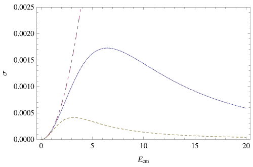
 . The dot-dashed (purple) line
depicts the case without asymptotic safety; the continuous (blue) and dashed (grey) line take into
account the running of the Planck mass, for two different values of the fixed point,
. The dot-dashed (purple) line
depicts the case without asymptotic safety; the continuous (blue) and dashed (grey) line take into
account the running of the Planck mass, for two different values of the fixed point,  and
and  respectively. Figure from [261*]; reproduced with permission from IOP.
 If we follow our earlier argument and use units of the running Planck mass, then the cross section as well
as the physically-relevant energy, in terms of the asymptotic quantities  , become constant at
the Planck scale. These indications for the existence of a minimal length scale in ASG are intriguing, in
particular because the dependence of the cross section on the energy offers a clean way to define a minimal
length scale from observable quantities, for example through the (square root of the) cross section at its
maximum value.
, become constant at
the Planck scale. These indications for the existence of a minimal length scale in ASG are intriguing, in
particular because the dependence of the cross section on the energy offers a clean way to define a minimal
length scale from observable quantities, for example through the (square root of the) cross section at its
maximum value.
However, it is not obvious how the above argument should be extended to interactions in which no
graviton exchange takes place. It has been argued on general grounds in [74*], that even in these cases the
dependence of the background on the energy of the exchange particle reduces the momentum transfer so
that the interaction would not probe distances below the Planck length and cross sections would
stagnate once the fixed-point regime has been reached, but the details require more study.
Recently, in [30] it has been argued that it is difficult to universally define the running of the
gravitational coupling because of the multitude of kinematic factors present at higher order. In
the simple example that we discussed here, the dependence of  on the
  seems like a
reasonable guess, but a cautionary note that this argument might not be possible to generalize is in
order.
seems like a
reasonable guess, but a cautionary note that this argument might not be possible to generalize is in
order.
3.6 Non-commutative geometry
Non-commutative geometry is both a modification of quantum mechanics and quantum field theory that arises within certain approaches towards quantum gravity, and a class of theories i n its own right. Thus, it could rightfully claim a place both in this section with motivations for a minimal length scale, and in Section 4 with applications. We will discuss the general idea of non-commutative geometries in the motivation because there is a large amount of excellent literature that covers the applications and phenomenology of non-commutative geometry. Thus, our treatment here will be very brief. For details, the interested reader is referred to [104*, 151*] and the many references therein.
String theory and M-theory are among the motivations to look at non-commutative geometries (see, e.g.,
the nice summary in [104*], section VII) and there have been indications that LQG may give rise to a
certain type of non-commutative geometry known as  -Poincaré. This approach has been very fruitful
and will be discussed in more detail later in Section 4.
-Poincaré. This approach has been very fruitful
and will be discussed in more detail later in Section 4.
The basic ingredient to non-commutative geometry is that, upon quantization, spacetime coordinates
 are associated to Hermitian operators
  that are non-commuting. The simplest way to do this is of
the form
that are non-commuting. The simplest way to do this is of
the form
![ν μ μν [ˆx , ˆx ] = i𝜃 . (155 )](article638x.gif)
 of dimension length squared is the deformation parameter
in this modification of quantum theory, known as the Poisson tensor. In the limit
of dimension length squared is the deformation parameter
in this modification of quantum theory, known as the Poisson tensor. In the limit  one
obtains ordinary spacetime. In this type of non-commutative geometry, the Poisson tensor is
not a dynamical field and defines a preferred frame and thereby breaks Lorentz invariance.
one
obtains ordinary spacetime. In this type of non-commutative geometry, the Poisson tensor is
not a dynamical field and defines a preferred frame and thereby breaks Lorentz invariance.
The deformation parameter enters here much like  in the commutation relation between position and
momentum; its physical interpretation is that of a smallest observable area in the
in the commutation relation between position and
momentum; its physical interpretation is that of a smallest observable area in the  -plane. The above
commutation relation leads to a minimal uncertainty among spacial coordinates of the form
-plane. The above
commutation relation leads to a minimal uncertainty among spacial coordinates of the form

 to be on the order of about the square of the Planck length,
though strictly speaking they are free parameters that have to be constrained by experiment.
to be on the order of about the square of the Planck length,
though strictly speaking they are free parameters that have to be constrained by experiment.
Quantization under the assumption of a non-commutative geometry can be extended from the
coordinates themselves to the algebra of functions  by using Weyl quantization. What one looks for is
a procedure
by using Weyl quantization. What one looks for is
a procedure  that assigns to each element
  in the algebra of functions
  a Hermitian
operator
a Hermitian
operator  in the algebra of operators
  . One does that by choosing a suitable
basis for elements of each algebra and then identifies them with each other. The most common
choice9
is to use a Fourier decomposition of the function
. One does that by choosing a suitable
basis for elements of each algebra and then identifies them with each other. The most common
choice9
is to use a Fourier decomposition of the function 


One can extend this isomorphism between the vector spaces to an algebra isomorphism by constructing
a new product, denoted  , that respects the map
  ,
,

 and
and  . From Eqs. (158*) and (159*) one finds the explicit expression
With the Campbell–Baker–Hausdorff formula
one has
and thus
This map can be inverted to
If one rewrites the
. From Eqs. (158*) and (159*) one finds the explicit expression
With the Campbell–Baker–Hausdorff formula
one has
and thus
This map can be inverted to
If one rewrites the 
![1 1- -1 1- eAeB = eA+B+ 2[A,B]+ 12[A,[A,B]]−12[B,[A,B ]]−24[B,[A,[A,B]]]+... (161 )](article661x.gif)


 -dependent factor into a differential operator acting on the plane-wave–basis, one can
also express this in the form
which is known as the Moyal–Weyl product [236].
-dependent factor into a differential operator acting on the plane-wave–basis, one can
also express this in the form
which is known as the Moyal–Weyl product [236].

The star product is a particularly useful way to handle non-commutative geometries, because one can continue to work with ordinary functions, one just has to keep in mind that they obey a modified product rule in the algebra. With that, one can build non-commutative quantum field theories by replacing normal products of fields in the Lagrangian with the star products.
To gain some insight into the way this product modifies the physics, it is useful to compute the star product with a delta function. For that, we rewrite Eq. (164*) as
And so, one finds the star product with a delta function to be In contrast to the normal product of functions, this describes a highly non-local operation. This non-locality, which is a characteristic property of the star product, is the most relevant feature of non-commutative geometry.

It is clear that the non-vanishing commutator by itself already introduces some notion of fundamentally-finite resolution, but there is another way to see how a minimal length comes into play in non-commutative geometry. To see that, we look at a Gaussian centered around zero. Gaussian distributions are of interest not only because they are widely used field configurations, but, for example, also because they may describe solitonic solutions in a potential [137*].
For simplicity, we will consider only two spatial dimensions and spatial commutativity, so then we have
where![[xˆi,xˆj ] = i𝜃𝜖ij, (168 )](article669x.gif)
 ,
,  is the totally antisymmetric tensor, and
  is the one remaining
free parameter in the Poisson tensor. This is a greatly simplified scenario, but it will suffice
here.
is the one remaining
free parameter in the Poisson tensor. This is a greatly simplified scenario, but it will suffice
here.
A normalized Gaussian in position space centered around zero with covariance 


 and
and  to
where
Back in position space this yields
Thus, if we multiply two Gaussians with
to
where
Back in position space this yields
Thus, if we multiply two Gaussians with 

 , the width of the product
  is larger than
  . In
fact, if we insert
. In
fact, if we insert  in Eq. (172*) and solve for
  , we see that a Gaussian with width
 squares to itself. Thus, since Gaussians with smaller width than
  have the effect to spread,
rather than to focus, the product, one can think of the Gaussian with width
have the effect to spread,
rather than to focus, the product, one can think of the Gaussian with width  as having a minimum
effective size.
as having a minimum
effective size.
In non-commutative quantum mechanics, even in more than one dimension, Gaussians with this
property constitute solutions to polynomial potentials with a mass term (for example for a cubic
potential this would be of the form  ) [137], because they
square to themselves, and so only higher powers continue to reproduce the original function.
) [137], because they
square to themselves, and so only higher powers continue to reproduce the original function.
3.7 Miscellaneous
Besides the candidate theories for quantum gravity so far discussed, there are also discrete approaches, reviewed, for example, in [203]. For these approaches, no general statement can be made with respect to the notion of a minimal length scale. Though one has lattice parameters that play the role of regulators, the goal is to eventually let the lattice spacing go to zero, leaving open the question of whether observables in this limit allow an arbitrarily good resolution of structures or whether the resolution remains bounded. One example of a discrete approach, where a minimal length appears, is the lattice approach by Greensite [139] (discussed also in Garay [120*]), in which the minimal length scale appears for much the same reason as it appears in the case of quantized conformal metric fluctuations discussed in Section 3.4. Even if the lattice spacing does not go to zero, it has been argued on general grounds in [60*] that discreteness does not necessarily imply a lower bound on the resolution of spatial distances.
One discrete approach in which a minimal length scale makes itself noticeable in yet another way are Causal Sets [290]. In this approach, one considers as fundamental the causal structure of spacetime, as realized by a partially-ordered, locally-finite set of points. This set, represented by a discrete sprinkling of points, replaces the smooth background manifold of general relativity. The “Hauptvermutung” (main conjecture) of the Causal Sets approach is that a causal set uniquely determines the macroscopic (coarse-grained) spacetime manifold. In full generality, this conjecture is so far unproven, though it has been proven in a limiting case [63]. Intriguingly, the causal sets approach to a discrete spacetime can preserve Lorentz invariance. This can be achieved by using not a regular but a random sprinkling of points; there is thus no meaningful lattice parameter in the ordinary sense. It has been shown in [62], that a Poisson process fulfills the desired property. This sprinkling has a finite density, which is in principle a parameter, but is usually assumed to be on the order of the Planckian density.
Another broad class of approaches to quantum gravity that we have so far not mentioned are emergent gravity scenarios, reviewed in [49, 284]. Also in these cases, there is no general statement that can be made about the existence of a minimal length scale. Since gravity is considered to be emergent (or induced), there has to enter some energy scale at which the true fundamental, non-gravitational, degrees of freedom make themselves noticeable. Yet, from this alone we do not know whether this also prevents a resolution of structures. In fact, in the absence of anything resembling spacetime, this might not even be a meaningful question to ask.
Giddings and Lippert [128, 129, 126] have proposed that the gravitational obstruction to test short distance probes should be translated into a fundamental limitation in quantum gravity distinct from the GUP. Instead of a modification of the uncertainty principle, fundamental limitations should arise due to strong gravitational (or other) dynamics, because the concept of locality is only approximate, giving rise to a ‘locality bound’ beyond which the notion of locality ceases to be meaningful. When the locality bound is violated, the usual field theory description of matter no longer accurately describes the quantum state and one loses the rationale for the usual Fock space description of the states; instead, one would have to deal with states able to describe a quantum black hole, whose full and proper quantum description is presently unknown.
Finally, we should mention an interesting recent approach by Dvali et al. that takes very seriously the previously-found bounds on the resolution of structures by black-hole formation [106*] and is partly related to the locality bound. However, rather than identifying a regime where quantum field theory breaks down and asking what quantum theory of gravity would allow one to consistently deal with strong curvature regimes, in Dvali et al.’s approach of ‘classicalization’, super-Planckian degrees of freedom cannot exist. On these grounds, it has been argued that classical gravity is in this sense UV-complete exactly because an arbitrarily good resolution of structures is physically impossible [105*].
3.8 Summary of motivations
In this section we have seen that there are many indications, from thought experiments as well as from different approaches to quantum gravity, that lead us to believe in a fundamental limit to the resolution of structure. But we have also seen that these limits appear in different forms.
The most commonly known form is a lower bound on spatial and temporal resolutions given by the Planck length, often realized by means of a GUP, in which the spatial uncertainty increases with the increase of the energy used to probe the structures. Such an uncertainty has been found in string theory, but we have also seen that this uncertainty does not seem to hold in string theory in general. Instead, in this particular approach to quantum gravity, it is more generally a spacetime uncertainty that still seems to hold. One also has to keep in mind here that this bound is given by the string scale, which may differ from the Planck scale. LQG and the simplified model for LQC give rise to bounds on the eigenvalues of the area and volume operator, and limit the curvature in the early universe to a Planckian value.
Thus, due to these different types of bounds, it is somewhat misleading to speak of a ‘minimal length,’ since in many cases a bound on the length itself does not exist, but only on the powers of spatio-temporal distances. Therefore, it is preferable to speak more generally of a ‘minimal length scale,’ and leave open the question of how this scale enters into the measurement of physical quantities.
 |
 |
 |
Living Rev. Relativity, 16 (2013), 2, doi:10.12942/lrr-2013-2, URL (accessed <date>): http://www.livingreviews.org/lrr-2013-2.
 This work is licensed under a Creative Commons License.
© The author(s), except where otherwise noted.
This work is licensed under a Creative Commons License.
© The author(s), except where otherwise noted.