11 Spinning Compact Binaries
The post-Newtonian templates have been developed so far for compact binary systems which can be described with great precision by point masses without spins. Here by spin, we mean the intrinsic (classical) angular momentum of the individual compact body. However, including the effects of spins is essential,
as the astrophysical evidence indicates that stellar-mass black holes [2, 390, 311, 227, 323] and
supermassive black holes [188, 101, 102] (see Ref. [364] for a review) can be generically close to maximally
spinning. The presence of spins crucially affects the dynamics of the binary, in particular leading to
orbital plane precession if they are not aligned with the orbital angular momentum (see for
instance [138, 8]), and thereby to strong modulations in the observed signal frequency and
phase.
of the individual compact body. However, including the effects of spins is essential,
as the astrophysical evidence indicates that stellar-mass black holes [2, 390, 311, 227, 323] and
supermassive black holes [188, 101, 102] (see Ref. [364] for a review) can be generically close to maximally
spinning. The presence of spins crucially affects the dynamics of the binary, in particular leading to
orbital plane precession if they are not aligned with the orbital angular momentum (see for
instance [138, 8]), and thereby to strong modulations in the observed signal frequency and
phase.
In recent years an important effort has been undertaken to compute spin effects to high post-Newtonian order in the dynamics and gravitational radiation of compact binaries:
- Dynamics. The goal is to obtain the equations of motion and related conserved integrals of the motion, the equations of precession of the spins, and the post-Newtonian metric in the near zone. For this step we need a formulation of the dynamics of particles with spins (either Lagrangian or Hamiltonian);
- Radiation. The mass and current radiative multipole moments, including tails and all hereditary effects, are to be computed. One then deduces the gravitational waveform and the fluxes, from which we compute the secular evolution of the orbital phase. This step requires plugging the previous dynamics into the general wave generation formalism of Part A.
We adopt a particular post-Newtonian counting for spin effects that actually refers to maximally
spinning black holes. In this convention the two spin variables  have the dimension of an
angular momentum multiplied by a factor
have the dimension of an
angular momentum multiplied by a factor  , and we pose

 is the mass of the compact body, and
  is the dimensionless spin parameter, which equals
one for maximally spinning Kerr black holes. Thus the spins
is the dimensionless spin parameter, which equals
one for maximally spinning Kerr black holes. Thus the spins  of the compact bodies can be considered
as “Newtonian” quantities [there are no
of the compact bodies can be considered
as “Newtonian” quantities [there are no  ’s in Eq. (366*)], and all spin effects will carry (at least) an
explicit
’s in Eq. (366*)], and all spin effects will carry (at least) an
explicit  factor with respect to non-spin effects. With this convention any post-Newtonian estimate is
expected to be appropriate (i.e., numerically correct) in the case of maximal rotation. One should keep in
mind that spin effects will be formally a factor
factor with respect to non-spin effects. With this convention any post-Newtonian estimate is
expected to be appropriate (i.e., numerically correct) in the case of maximal rotation. One should keep in
mind that spin effects will be formally a factor  smaller for non-maximally spinning objects such as
neutron stars; thus in this case a given post-Newtonian computation will actually be a factor
smaller for non-maximally spinning objects such as
neutron stars; thus in this case a given post-Newtonian computation will actually be a factor  more
accurate.
more
accurate.
As usual we shall make a distinction between spin-orbit (SO) effects, which are linear in the spins, and spin-spin (SS) ones, which are quadratic. In this article we shall especially review the SO effects as they play the most important role in gravitational wave detection and parameter estimation. As we shall see a good deal is known on spin effects (both SO and SS), but still it will be important in the future to further improve our knowledge of the waveform and gravitational-wave phasing, by computing still higher post-Newtonian SO and SS terms, and to include at least the dominant spin-spin-spin (SSS) effect [305*]. For the computations of SSS and even SSSS effects see Refs. [246, 245, 296, 305, 413].
The SO effects have been known at the leading level since the seminal works of Tulczyjew [411*, 412*], Barker & O’Connell [27*, 28*] and Kidder et al. [275*, 271*]. With our post-Newtonian counting such leading level corresponds to the 1.5PN order. The SO terms have been computed to the next-to-leading level which corresponds to 2.5PN order in Refs. [394*, 194*, 165*, 292*, 352*, 241*] for the equations of motion or dynamics, and in Refs. [53*, 54*] for the gravitational radiation field. Note that Refs. [394, 194, 165*, 241*] employ traditional post-Newtonian methods (both harmonic-coordinates and Hamiltonian), but that Refs. [292, 352] are based on the effective field theory (EFT) approach. The next-to-next-to-leading SO level corresponding to 3.5PN order has been obtained in Refs. [242, 244] using the Hamiltonian method for the equations of motion, in Ref. [297] using the EFT, and in Refs. [307*, 90*] using the harmonic-coordinates method. Here we shall focus on the harmonic-coordinates approach [307*, 90*, 89*, 306*] which is in fact best formulated using a Lagrangian, see Section 11.1. With this approach the next-to-next-to-leading SO level was derived not only for the equations of motion including precession, but also for the radiation field (energy flux and orbital phasing) [89*, 306*]. An analytic solution for the SO precession effects will be presented in Section 11.2. Note that concerning the radiation field the highest known SO level actually contains specific tail-induced contributions at 3PN [54*] and 4PN [306*] orders, see Section 11.3.
The SS effects are known at the leading level corresponding to 2PN order from Barker &
O’Connell [27, 28] in the equations of motion (see [271*, 351*, 110] for subsequent derivations), and from
Refs. [275, 271*] in the radiation field. Next-to-leading SS contributions are at 3PN order and have been
obtained with Hamiltonian [387, 389*, 388, 247, 241], EFT [354, 356, 355, 293, 299] and
harmonic-coordinates [88*] techniques (with [88] obtaining also the next-to-leading SS terms in the
gravitational-wave flux). With SS effects in a compact binary system one must make a distinction between
the spin squared terms, involving the coupling between the two same spins  or
or  , and the interaction
terms, involving the coupling between the two different spins
, and the interaction
terms, involving the coupling between the two different spins  and
and  . The spin-squared terms
  and
and  arise due to the effects on the dynamics of the quadrupole moments of the compact
bodies that are induced by their spins [347]. They have been computed through 2PN order in
the fluxes and orbital phase in Refs. [217, 218*, 314]. The interaction terms
arise due to the effects on the dynamics of the quadrupole moments of the compact
bodies that are induced by their spins [347]. They have been computed through 2PN order in
the fluxes and orbital phase in Refs. [217, 218*, 314]. The interaction terms  can be
computed using a simple pole-dipole formalism like the one we shall review in Section 11.1. The
interaction terms
can be
computed using a simple pole-dipole formalism like the one we shall review in Section 11.1. The
interaction terms  between different spins have been derived to next-to-next-to-leading
4PN order for the equations of motion in Refs. [294, 298] (EFT) and [243] (Hamiltonian). In
this article we shall generally neglect the SS effects and refer for these to the literature quoted
above.
between different spins have been derived to next-to-next-to-leading
4PN order for the equations of motion in Refs. [294, 298] (EFT) and [243] (Hamiltonian). In
this article we shall generally neglect the SS effects and refer for these to the literature quoted
above.
11.1 Lagrangian formalism for spinning point particles
Some necessary material for constructing a Lagrangian for a spinning point particle in curved spacetime is presented here. The formalism is issued from early works [239*, 19*] and has also been developed in the context of the EFT approach [351*]. Variants and alternatives (most importantly the associated Hamiltonian formalism) can be found in Refs. [389, 386, 25]. The formalism yields for the equations of motion of spinning particles and the equations of precession of the spins the classic results known in general relativity [411*, 412*, 310*, 331*, 135*, 409*, 179*].
Let us consider a single spinning point particle moving in a given curved background metric
 . The particle follows the worldline
  , with tangent four-velocity
  ,
where
,
where  is a parameter along the representative worldline. In a first stage we do not require
that the four-velocity be normalized; thus
is a parameter along the representative worldline. In a first stage we do not require
that the four-velocity be normalized; thus  needs not be the proper time elapsed along the
worldline. To describe the internal degrees of freedom associated with the particle’s spin, we
introduce a moving orthonormal tetrad
needs not be the proper time elapsed along the
worldline. To describe the internal degrees of freedom associated with the particle’s spin, we
introduce a moving orthonormal tetrad  along the trajectory, which defines a “body-fixed”
frame.77
The rotation tensor
along the trajectory, which defines a “body-fixed”
frame.77
The rotation tensor  associated with the tetrad is defined by

 is the covariant derivative with respect to the parameter
  along the worldline;
equivalently, we have
Because of the normalization of the tetrad the rotation tensor is antisymmetric:
along the worldline;
equivalently, we have
Because of the normalization of the tetrad the rotation tensor is antisymmetric: 
 .
.
We look for an action principle for the spinning particle. Following Refs. [239*, 351] and the general spirit of effective field theories, we require the following symmetries to hold:
- The action is a covariant scalar, i.e., behaves as a scalar with respect to general space-time diffeomorphisms;
- It is a global Lorentz scalar, i.e., stays invariant under an arbitrary change of the tetrad vectors:
 where
where  is a constant Lorentz matrix;
- It is reparametrization-invariant, i.e., its form is independent of the parameter
 used to
follow the particle’s worldline.
used to
follow the particle’s worldline.
In addition to these symmetries we need to specify the dynamical degrees of freedom: These are chosen to be
the particle’s position  and the tetrad
  . Furthermore we restrict ourselves to a Lagrangian
depending only on the four-velocity
. Furthermore we restrict ourselves to a Lagrangian
depending only on the four-velocity  , the rotation tensor
  , and the metric
  . Thus, the
postulated action is of the type
. Thus, the
postulated action is of the type
![[ ] ∫ +∞ ( ) I yα,eA α = d τL u α,ωαβ,gαβ . (369 ) −∞](article2835x.gif)
As it is written in (369*), i.e., depending only on Lorentz scalars,  is automatically a Lorentz scalar.
By performing an infinitesimal coordinate transformation, one easily sees that the requirement that the
Lagrangian be a covariant scalar specifies its dependence on the metric to be such that (see e.g., Ref. [19])
is automatically a Lorentz scalar.
By performing an infinitesimal coordinate transformation, one easily sees that the requirement that the
Lagrangian be a covariant scalar specifies its dependence on the metric to be such that (see e.g., Ref. [19])

 and the antisymmetric spin tensor
  by
by
Note that the right-hand side of Eq. (370*) is necessarily symmetric by exchange of the indices  and
and
 . Finally, imposing the invariance of the action (369*) by reparametrization of the worldline, we find
that the Lagrangian must be a homogeneous function of degree one in the velocity
. Finally, imposing the invariance of the action (369*) by reparametrization of the worldline, we find
that the Lagrangian must be a homogeneous function of degree one in the velocity  and
rotation tensor
and
rotation tensor  . Applying Euler’s theorem to the function
  immediately gives

 and
and  must be reparametrization invariant. Note that, at this
stage, their explicit expressions are not known. They will be specified only when a spin supplementary
condition is imposed, see Eq. (379*) below.
must be reparametrization invariant. Note that, at this
stage, their explicit expressions are not known. They will be specified only when a spin supplementary
condition is imposed, see Eq. (379*) below.
We now investigate the unconstrained variations of the action (369*) with respect to the dynamical
variables  ,
,  and the metric. First, we vary it with respect to the tetrad
  while keeping the
position
while keeping the
position  fixed. A worry is that we must have a way to distinguish intrinsic variations of the tetrad
from variations which are induced by a change of the metric
fixed. A worry is that we must have a way to distinguish intrinsic variations of the tetrad
from variations which are induced by a change of the metric  . This is conveniently solved by
decomposing the variation
. This is conveniently solved by
decomposing the variation  according to

![αβ A [α β] δ𝜃 ≡ e δeA](article2856x.gif) , and where the corresponding
symmetric part is simply given by the variation of the metric, i.e.
, and where the corresponding
symmetric part is simply given by the variation of the metric, i.e.  . Then we can
consider the independent variations
. Then we can
consider the independent variations  and
and  . Varying with respect to
  , but holding the
metric fixed, gives the equation of spin precession which is found to be
or, alternatively, using the fact that the right-hand side of Eq. (370*) is symmetric,
We next vary with respect to the particle’s position
, but holding the
metric fixed, gives the equation of spin precession which is found to be
or, alternatively, using the fact that the right-hand side of Eq. (370*) is symmetric,
We next vary with respect to the particle’s position 

 while holding the tetrad
  fixed.
Operationally, this means that we have to parallel-transport the tetrad along the displacement vector, i.e.,
to impose
A simple way to derive the result is to use locally inertial coordinates, such that the Christoffel symbols
fixed.
Operationally, this means that we have to parallel-transport the tetrad along the displacement vector, i.e.,
to impose
A simple way to derive the result is to use locally inertial coordinates, such that the Christoffel symbols

 along the particle’s worldline
  ; then, Eq. (376*) gives
  .
The variation leads then to the well-known Mathisson–Papapetrou [310*, 331*, 135*] equation of motion
which involves the famous coupling of the spin tensor to the Riemann
curvature.78
With a little more work, the equation of motion (377*) can also be derived using an arbitrary coordinate
system, making use of the parallel transport equation (376*). Finally, varying with respect to the metric
while keeping
.
The variation leads then to the well-known Mathisson–Papapetrou [310*, 331*, 135*] equation of motion
which involves the famous coupling of the spin tensor to the Riemann
curvature.78
With a little more work, the equation of motion (377*) can also be derived using an arbitrary coordinate
system, making use of the parallel transport equation (376*). Finally, varying with respect to the metric
while keeping 
 , gives the stress-energy tensor of the spinning particle. We must again take into
account the scalarity of the action, as imposed by Eq. (370*). We obtain the standard pole-dipole
result [411*, 412*, 310, 331, 135, 409, 179]:
where
, gives the stress-energy tensor of the spinning particle. We must again take into
account the scalarity of the action, as imposed by Eq. (370*). We obtain the standard pole-dipole
result [411*, 412*, 310, 331, 135, 409, 179]:
where 
 denotes the four-dimensional Dirac function. It can easily be checked that the covariant
conservation law
denotes the four-dimensional Dirac function. It can easily be checked that the covariant
conservation law  holds as a consequence of the equation of motion (377*) and the equation of
spin precession (375*).
holds as a consequence of the equation of motion (377*) and the equation of
spin precession (375*).
Up to now we have considered unconstrained variations of the action (369*), describing the particle’s
internal degrees of freedom by the six independent components of the tetrad  (namely a
  matrix subject to the 10 constraints
  ). To correctly account for the number of degrees of
freedom associated with the spin, we must impose three supplementary spin conditions (SSC). Several
choices are possible for a sensible SSC. Notice that in the case of extended bodies the choice of a SSC
corresponds to the choice of a central worldline inside the body with respect to which the spin angular
momentum is defined (see Ref. [271*] for a discussion). Here we adopt the Tulczyjew covariant
SSC [411, 412]
). To correctly account for the number of degrees of
freedom associated with the spin, we must impose three supplementary spin conditions (SSC). Several
choices are possible for a sensible SSC. Notice that in the case of extended bodies the choice of a SSC
corresponds to the choice of a central worldline inside the body with respect to which the spin angular
momentum is defined (see Ref. [271*] for a discussion). Here we adopt the Tulczyjew covariant
SSC [411, 412]

 associated with the spin tensor
by79
where we have defined the mass of the particle by
associated with the spin tensor
by79
where we have defined the mass of the particle by 
 . By contracting Eq. (375*) with
  and using the equation of motion (377*), one obtains
where we denote
and using the equation of motion (377*), one obtains
where we denote 
 . By further contracting Eq. (381*) with
  we obtain an explicit
expression for
we obtain an explicit
expression for  , which can then be substituted back into (381*) to provide the relation linking the
four-momentum
, which can then be substituted back into (381*) to provide the relation linking the
four-momentum  to the four-velocity
  . It can be checked using (379*) and (381*) that the
mass of the particle is constant along the particle’s trajectory:
. It can be checked using (379*) and (381*) that the
mass of the particle is constant along the particle’s trajectory:  . Furthermore
the four-dimensional magnitude
. Furthermore
the four-dimensional magnitude  of the spin defined by
  is also conserved:
 .
.
Henceforth we shall restrict our attention to spin-orbit (SO) interactions, which are linear in
the spins. We shall also adopt for the parameter  along the particle’s worldline the proper
time
along the particle’s worldline the proper
time  , so that
  . Neglecting quadratic spin-spin (SS) and
higher-order interactions, the linear momentum is simply proportional to the normalized four-velocity:
. Neglecting quadratic spin-spin (SS) and
higher-order interactions, the linear momentum is simply proportional to the normalized four-velocity:
 . Hence, from Eq. (375*) we deduce that
  . The equation for the
spin covariant vector
. The equation for the
spin covariant vector  then reduces at linear order to


 remainders.
In applications (e.g., the construction of gravitational wave templates for the compact binary inspiral) it
is very useful to introduce new spin variables that are designed to have a conserved three-dimensional
Euclidean norm (numerically equal to  ). Using conserved-norm spin vector variables is indeed the most
natural choice when considering the dynamics of compact binaries reduced to the frame of the center of
mass or to circular orbits [90*]. Indeed the evolution equations of such spin variables reduces, by
construction, to ordinary precession equations, and these variables are secularly constant (see
Ref. [423*]).
). Using conserved-norm spin vector variables is indeed the most
natural choice when considering the dynamics of compact binaries reduced to the frame of the center of
mass or to circular orbits [90*]. Indeed the evolution equations of such spin variables reduces, by
construction, to ordinary precession equations, and these variables are secularly constant (see
Ref. [423*]).
A standard, general procedure to define a (Euclidean) conserved-norm spin spatial vector consists of
projecting the spin covector  onto an orthonormal tetrad
  , which leads to the four scalar
components (
, which leads to the four scalar
components ( )
)

 ,80
the time component tetrad projection
,80
the time component tetrad projection  vanishes because of the orthogonality condition (383*). We have
seen that
vanishes because of the orthogonality condition (383*). We have
seen that  is conserved along the trajectory; because of (383*) we can rewrite this as
 , in which we have introduced the projector
  onto the spatial
hypersurface orthogonal to
onto the spatial
hypersurface orthogonal to  . From the orthonormality of the tetrad and our choice
  , we
have
, we
have  in which
  refer to the spatial values of the tetrad indices,
i.e.,
refer to the spatial values of the tetrad indices,
i.e.,  and
and  . Therefore the conservation law
  becomes
which is indeed the relation defining a Euclidean conserved-norm spin variable
becomes
which is indeed the relation defining a Euclidean conserved-norm spin variable

 .81
However, note that the choice of the spin variable
.81
However, note that the choice of the spin variable  is still somewhat arbitrary, since a rotation of
the tetrad vectors can freely be performed. We refer to [165, 90*] for the definition of some
“canonical” choice for the tetrad in order to fix this residual freedom. Such choice presents
the advantage of providing a unique determination of the conserved-norm spin variable in a
given gauge. This canonical choice will be the one adopted in all explicit results presented in
Section 11.3.
is still somewhat arbitrary, since a rotation of
the tetrad vectors can freely be performed. We refer to [165, 90*] for the definition of some
“canonical” choice for the tetrad in order to fix this residual freedom. Such choice presents
the advantage of providing a unique determination of the conserved-norm spin variable in a
given gauge. This canonical choice will be the one adopted in all explicit results presented in
Section 11.3.
The evolution equation (382*) for the original spin variable  now translates into an ordinary
precession equation for the tetrad components
now translates into an ordinary
precession equation for the tetrad components  , namely

 is related to the tetrad components
  of the rotation tensor defined
in (368*) by
of the rotation tensor defined
in (368*) by  where we pose
  , remembering the redshift variable (276*). The
antisymmetric character of the matrix
, remembering the redshift variable (276*). The
antisymmetric character of the matrix  guaranties that
  satisfies the Euclidean precession
equation
where we denote
satisfies the Euclidean precession
equation
where we denote 
 , and
, and  with
with  . As a consequence of (387*) the spin
has a conserved Euclidean norm:
. As a consequence of (387*) the spin
has a conserved Euclidean norm:  . From now on we shall no longer make any distinction between
the spatial tetrad indices
. From now on we shall no longer make any distinction between
the spatial tetrad indices  and the ordinary spatial indices
  which are raised and lowered with
the Kronecker metric. Explicit results for the equations of motion and gravitational wave templates will be
given in Sections 11.2 and 11.3 using the canonical choice for the conserved-norm spin variable
which are raised and lowered with
the Kronecker metric. Explicit results for the equations of motion and gravitational wave templates will be
given in Sections 11.2 and 11.3 using the canonical choice for the conserved-norm spin variable
 .
.
11.2 Equations of motion and precession for spin-orbit effects
The previous formalism can be generalized to self-gravitating systems consisting of two (or more generally N) spinning point particles. The metric generated by the system of particles, interacting only through gravitation, is solution of the Einstein field equations (18*) with stress-energy tensor given by the sum of the individual stress-energy tensors (378*) for each particles. The equations of motion of the particles are given by the Mathisson–Papapetrou equations (377*) with “self-gravitating” metric evaluated at the location of the particles thanks to a regularization procedure (see Section 6). The precession equations of each of the spins are given by
where
 labels the particles. The spin variables
  are the conserved-norm spins defined in Section 11.1. In
the following it is convenient to introduce two combinations of the individuals spins defined by (with
are the conserved-norm spins defined in Section 11.1. In
the following it is convenient to introduce two combinations of the individuals spins defined by (with  and
and
 )82
)82
We shall investigate the case where the binary’s orbit is quasi-circular, i.e., whose radius is constant
apart from small perturbations induced by the spins (as usual we neglect the gravitational
radiation damping effects). We denote by  and
and  the relative position and
velocity.83
We introduce an orthonormal moving triad
the relative position and
velocity.83
We introduce an orthonormal moving triad  defined by the unit separation vector
  (with
(with  ) and the unit normal
  to the instantaneous orbital plane given by
  ;
the orthonormal triad is then completed by
;
the orthonormal triad is then completed by  . Those vectors are represented on Figure 4*, which
shows the geometry of the system. The orbital frequency
. Those vectors are represented on Figure 4*, which
shows the geometry of the system. The orbital frequency  is defined for general orbits, not necessarily
circular, by
is defined for general orbits, not necessarily
circular, by  where
where  represents the derivative of
  with respect to the
coordinate time
with respect to the
coordinate time  . The general expression for the relative acceleration
  decomposed in the
moving basis
decomposed in the
moving basis  is
is

 of the orbit defined by
  . Next
we impose the restriction to quasi-circular precessing orbits which is defined by the conditions
. Next
we impose the restriction to quasi-circular precessing orbits which is defined by the conditions
 and
and  so that
  ; see Eqs. (227). Then
  represents the direction of the velocity, and the precession frequency
  is proportional to the variation of
 in the direction of the velocity. In this way we find that the equations of the relative motion in the
frame of the center-of-mass are
Since we neglect the radiation reaction damping there is no component of the acceleration along
in the direction of the velocity. In this way we find that the equations of the relative motion in the
frame of the center-of-mass are
Since we neglect the radiation reaction damping there is no component of the acceleration along 
 . This
equation represents the generalization of Eq. (226*) for spinning quasi-circular binaries with
no radiation reaction. The orbital frequency
. This
equation represents the generalization of Eq. (226*) for spinning quasi-circular binaries with
no radiation reaction. The orbital frequency  will contain spin effects in addition to the
non-spin terms given by (228), while the precessional frequency
will contain spin effects in addition to the
non-spin terms given by (228), while the precessional frequency  will entirely be due to
spins.
will entirely be due to
spins.
Here we report the latest results for the spin-orbit (SO) contributions into these quantities at the
next-to-next-to-leading level corresponding to 3.5PN order [307*, 90*]. We project out the spins on
the moving orthonormal basis, defining  and similarly for
  . We
have
. We
have
which has to be added to the non-spin terms (228) up to 3.5PN order. We recall that the ordering
post-Newtonian parameter is  . On the other hand the next-to-next-to-leading SO effects into the
precessional frequency read
. On the other hand the next-to-next-to-leading SO effects into the
precessional frequency read
where this time the ordering post-Newtonian parameter is  . The SO terms at the
same level in the conserved energy associated with the equations of motion will be given in
Eq. (415) below. In order to complete the evolution equations for quasi-circular orbits we need
also the precession vectors
. The SO terms at the
same level in the conserved energy associated with the equations of motion will be given in
Eq. (415) below. In order to complete the evolution equations for quasi-circular orbits we need
also the precession vectors  of the two spins as defined by Eq. (388*). These are given
by
of the two spins as defined by Eq. (388*). These are given
by
We obtain  from
from  simply by exchanging the masses,
  .
At the linear SO level the precession vectors
.
At the linear SO level the precession vectors  are independent of the
spins.84
are independent of the
spins.84
We now investigate an analytical solution for the dynamics of compact spinning binaries on quasi-circular orbits, including the effects of spin precession [54*, 306*]. This solution will be valid whenever the radiation reaction effects can be neglected, and is restricted to the linear SO level.
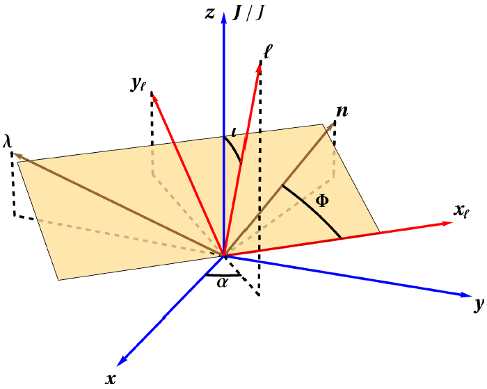
 ; (ii) the instantaneous
orbital plane which is described by the orthonormal basis
; (ii) the instantaneous
orbital plane which is described by the orthonormal basis  ; (iii) the moving triad
 and the associated three Euler angles
  ,
,  and
and  ; (v) the direction of the total
angular momentum
; (v) the direction of the total
angular momentum  which coincides with the
  –direction. Dashed lines show projections into
the
–direction. Dashed lines show projections into
the  –
– plane.
 In the following, we will extensively employ the total angular momentum of the system,
that we denote by  , and which is conserved when radiation-reaction effects are neglected,

 as the sum of the orbital angular momentum
  and
of the two spins,85
This split between
and
of the two spins,85
This split between 
 and
and  is specified by our choice of spin variables, here the
conserved-norm spins defined in Section 11.1. Note that although
is specified by our choice of spin variables, here the
conserved-norm spins defined in Section 11.1. Note that although  is called the “orbital”
angular momentum, it actually includes both non-spin and spin contributions. We refer to
Eq. (4.7) in [90*] for the expression of
is called the “orbital”
angular momentum, it actually includes both non-spin and spin contributions. We refer to
Eq. (4.7) in [90*] for the expression of  at the next-to-next-to-leading SO level for quasi-circular
orbits.
at the next-to-next-to-leading SO level for quasi-circular
orbits.
Our solution will consist of some explicit expressions for the moving triad  at the SO level in
the conservative dynamics for quasi-circular orbits. With the previous definitions of the orbital frequency
at the SO level in
the conservative dynamics for quasi-circular orbits. With the previous definitions of the orbital frequency
 and the precessional frequency
  we have the following system of equations for the time evolution of
the triad vectors,
we have the following system of equations for the time evolution of
the triad vectors,
Equivalently, introducing the orbital rotation vector  and spin precession vector
  ,
these equations can be elegantly written as
,
these equations can be elegantly written as
Next we introduce a fixed (inertial) orthonormal basis  as follows:
  is defined to be the
normalized value
is defined to be the
normalized value  of the total angular momentum
  ;
;  is orthogonal to the plane spanned by
  and the direction
  of the detector as seen from the source (notation of Section 3.1) and is
defined by
of the detector as seen from the source (notation of Section 3.1) and is
defined by  ; and
; and  completes the triad – see Figure 4*. Then, we introduce
the standard spherical coordinates
completes the triad – see Figure 4*. Then, we introduce
the standard spherical coordinates  of the vector
  measured in the inertial basis
 . Since
  is the angle between the total and orbital angular momenta, we have

 . The angles
  are referred to as the precession angles.
We now derive from the time evolution of our triad vectors those of the precession angles  , and of
an appropriate phase
, and of
an appropriate phase  that specifies the position of
  with respect to some reference direction in the
orbital plane denoted
with respect to some reference direction in the
orbital plane denoted  . Following Ref. [13], we pose
such that  forms an orthonormal basis. The motion takes place in the instantaneous
orbital plane spanned by
forms an orthonormal basis. The motion takes place in the instantaneous
orbital plane spanned by  and
and  , and the phase angle
  is such that (see Figure 4*):

from which we deduce
Combining Eqs. (402*) with (399*) we also get By identifying the right-hand sides of (397) with the time-derivatives of the relations (401) we obtain the following system of equations for the variations of

 ,
,  and
and  ,
,
On the other hand, using the decompositon of the total angular momentum (396*) together with the fact
that the components of  projected along
  and
and  are of the order
  , see e.g., Eq. (4.7) in
Ref. [90*], we deduce that
, see e.g., Eq. (4.7) in
Ref. [90*], we deduce that  is itself a small quantity of order
  . Since we also have
 , we conclude by direct integration of the sum of Eqs. (404a) and (404c) that


 the value of the carrier phase at some arbitrary initial time
  . An important point we have
used when integrating (406*) is that the orbital frequency
. An important point we have
used when integrating (406*) is that the orbital frequency  is constant at linear order in the
spins. Indeed, from Eq. (392) we see that only the components of the conserved-norm spin
vectors along
is constant at linear order in the
spins. Indeed, from Eq. (392) we see that only the components of the conserved-norm spin
vectors along  can contribute to
  at linear order. As we show in Eq. (409c) below, these
components are in fact constant at linear order in spins. Thus we can treat
at linear order. As we show in Eq. (409c) below, these
components are in fact constant at linear order in spins. Thus we can treat  as a constant for our
purpose.
as a constant for our
purpose.
The combination  being known by Eq. (405*), we can further express the precession angles
  and
and  at linear order in spins in terms of the components
  and
and  ; from Eqs. (399*) and (403*):
where we denote by  the norm of the non-spin (NS) part of the orbital angular momentum
 .
.
It remains to obtain the explicit time variation of the components of the two individual spins  ,
,
 and
and  (with
(with  ). Using Eqs. (407) together with the decomposition (396*) and
the explicit expression of
). Using Eqs. (407) together with the decomposition (396*) and
the explicit expression of  in Ref. [90*], we shall then be able to obtain the explicit time
variation of the precession angles
in Ref. [90*], we shall then be able to obtain the explicit time
variation of the precession angles  and phase
  . Combining (388*) and (397) we obtain
where  is the norm of the precession vector of the
  -th spin as given by (394), and the precession
frequency
-th spin as given by (394), and the precession
frequency  is explicitly given by (393). At linear order in spins these equations translate into
We see that, as stated before, the spin components along  are constant, and so is the orbital
frequency
are constant, and so is the orbital
frequency  given by (392). At the linear SO level, the equations (409) can be decoupled and integrated
as
given by (392). At the linear SO level, the equations (409) can be decoupled and integrated
as
Here  and
and  denote two quantities for each spins, that are constant up to terms
  .
The phase of the projection perpendicular to the direction
.
The phase of the projection perpendicular to the direction  of each of the spins is given by

 is the constant initial phase at the reference time
  .
.
Finally we can give in an explicit way, to linear SO order, the triad  in terms of
some reference triad
in terms of
some reference triad  at the reference time
  in Eqs. (411*) and (406*). The
best way to express the result is to introduce the complex null vector
in Eqs. (411*) and (406*). The
best way to express the result is to introduce the complex null vector  and
its complex conjuguate
and
its complex conjuguate  ; the normalization is chosen so that
  . We obtain
The precession effects in the dynamical solution for the evolution of the basis vectors  are
given by the second terms in these equations. They depend only in the combination
are
given by the second terms in these equations. They depend only in the combination  and its
complex conjugate
and its
complex conjugate  , which follows from Eqs. (407) and the known spin and non-spin
contributions to the total angular momentum
, which follows from Eqs. (407) and the known spin and non-spin
contributions to the total angular momentum  . One can check that precession effects in the above
dynamical solution (412) for the moving triad start at order
. One can check that precession effects in the above
dynamical solution (412) for the moving triad start at order  .
.
11.3 Spin-orbit effects in the gravitational wave flux and orbital phase
Like in Section 9 our main task is to control up to high post-Newtonian order the mass and current radiative
multipole moments  and
and  which parametrize the asymptotic waveform and gravitational fluxes far
away from the source, cf. Eqs. (66) – (68). The radiative multipole moments are in turn related to the source
multipole moments
which parametrize the asymptotic waveform and gravitational fluxes far
away from the source, cf. Eqs. (66) – (68). The radiative multipole moments are in turn related to the source
multipole moments  and
and  through complicated relationships involving tails and related effects; see e.g.,
Eqs. (76).86
through complicated relationships involving tails and related effects; see e.g.,
Eqs. (76).86
The source moments have been expressed in Eqs. (123) in terms of some source densities  ,
,  and
and
 defined from the components of the post-Newtonian expansion of the pseudo-tensor,
denoted
defined from the components of the post-Newtonian expansion of the pseudo-tensor,
denoted  . To lowest order the (PN expansion of the) pseudo-tensor reduces to the matter
tensor
. To lowest order the (PN expansion of the) pseudo-tensor reduces to the matter
tensor  which has compact support, and the source densities
  ,
,  ,
,  reduce to
the compact support quantities
reduce to
the compact support quantities  ,
, 
 given by Eqs. (145). Now, computing spin
effects, the matter tensor
given by Eqs. (145). Now, computing spin
effects, the matter tensor  has been found to be given by (378*) in the framework of the
pole-dipole approximation suitable for SO couplings (and sufficient also for SS interactions between
different spins). Here, to give a flavor of the computation, we present the lowest order spin
contributions (necessarily SO) to the general mass and current source multipole moments (
has been found to be given by (378*) in the framework of the
pole-dipole approximation suitable for SO couplings (and sufficient also for SS interactions between
different spins). Here, to give a flavor of the computation, we present the lowest order spin
contributions (necessarily SO) to the general mass and current source multipole moments ( ):
):
Paralleling the similar expressions (304) for the Newtonian approximation to the source moments in the
non-spin case, we posed  with
with  [see also Eqs. (305)]. In Eqs. (413)
we employ the notation (389) for the two spins and the ordinary cross product
[see also Eqs. (305)]. In Eqs. (413)
we employ the notation (389) for the two spins and the ordinary cross product  of Euclidean vectors.
Thus, the dominant level of spins is at the 1.5PN order in the mass-type moments
of Euclidean vectors.
Thus, the dominant level of spins is at the 1.5PN order in the mass-type moments  , but only at the
0.5PN order in the current-type moments
, but only at the
0.5PN order in the current-type moments  . It is then evident that the spin part of the current-type
moments will always dominate over that of the mass-type moments. We refer to [53*, 89*] for higher order
post-Newtonian expressions of the source moments. If we insert the expressions (413) into tail
integrals like (76), we find that some spin contributions originate from tails starting at the 3PN
order [54*].
. It is then evident that the spin part of the current-type
moments will always dominate over that of the mass-type moments. We refer to [53*, 89*] for higher order
post-Newtonian expressions of the source moments. If we insert the expressions (413) into tail
integrals like (76), we find that some spin contributions originate from tails starting at the 3PN
order [54*].
Finally, skipping details, we are left with the following highest-order known result for the SO contributions to the gravitational wave energy flux, which is currently 4PN order [53, 89*, 306]:87
We recall that  and
and  , with
  and
and  denoting the combinations (389), and
the individual spins are the specific conserved-norm spins that have been introduced in Section 11.1. The
result (414) superposes to the non-spin contributions given by Eq. (314). Satisfyingly it is in complete
agreement in the test-mass limit where
denoting the combinations (389), and
the individual spins are the specific conserved-norm spins that have been introduced in Section 11.1. The
result (414) superposes to the non-spin contributions given by Eq. (314). Satisfyingly it is in complete
agreement in the test-mass limit where  with the result of black-hole perturbation theory on a Kerr
background obtained in Ref. [396].
with the result of black-hole perturbation theory on a Kerr
background obtained in Ref. [396].
Finally we can compute the spin effects in the time evolution of the binary’s orbital frequency  . We
rely as in Section 9 on the equation (295*) balancing the total emitted energy flux
. We
rely as in Section 9 on the equation (295*) balancing the total emitted energy flux  with the variation of
the binary’s center-of-mass energy
with the variation of
the binary’s center-of-mass energy  . The non-spin contributions in
  have been provided for
quasi-circular binaries in Eq. (232); the SO contributions to next-to-next-to-leading order are given
by [307, 90]
have been provided for
quasi-circular binaries in Eq. (232); the SO contributions to next-to-next-to-leading order are given
by [307, 90]
Using  and
and  expressed as functions of the orbital frequency
  (through
  ) and of the spin
variables (through
) and of the spin
variables (through  and
and  ), we transform the balance equation into

However, in writing the latter equation it is important to justify that the spin quantities  and
and  are secularly constant, i.e., do not evolve on a gravitational radiation reaction time scale so we can
neglect their variations when taking the time derivative of Eq. (415). Fortunately, this is the case
of the conserved-norm spin variables, as proved in Ref. [423] up to relative 1PN order, i.e.,
considering radiation reaction effects up to 3.5PN order. Furthermore this can also be shown
from the following structural general argument valid at linear order in spins [54, 89]. In the
center-of-mass frame, the only vectors at our disposal, except for the spins, are
are secularly constant, i.e., do not evolve on a gravitational radiation reaction time scale so we can
neglect their variations when taking the time derivative of Eq. (415). Fortunately, this is the case
of the conserved-norm spin variables, as proved in Ref. [423] up to relative 1PN order, i.e.,
considering radiation reaction effects up to 3.5PN order. Furthermore this can also be shown
from the following structural general argument valid at linear order in spins [54, 89]. In the
center-of-mass frame, the only vectors at our disposal, except for the spins, are  and
and  .
Recalling that the spin vectors are pseudovectors regarding parity transformation, we see that
the only way SO contributions can enter scalars such as the energy
.
Recalling that the spin vectors are pseudovectors regarding parity transformation, we see that
the only way SO contributions can enter scalars such as the energy  or the flux
  is
through the mixed products
is
through the mixed products  , i.e., through the components
  . Now, the same
reasoning applies to the precession vectors
. Now, the same
reasoning applies to the precession vectors  in Eqs. (388*): They must be pseudovectors,
and, at linear order in spin, they must only depend on
in Eqs. (388*): They must be pseudovectors,
and, at linear order in spin, they must only depend on  and
and  ; so that they must be
proportional to
; so that they must be
proportional to  , as can be explicitly seen for instance in Eq. (394). Now, the time derivative of
the components along
, as can be explicitly seen for instance in Eq. (394). Now, the time derivative of
the components along  of the spins are given by
  . The
second term vanishes because
. The
second term vanishes because  , and since
  , we obtain that
  is
constant at linear order in the spins. We have already met an instance of this important fact in
Eq. (409c). This argument is valid at any post-Newtonian order and for general orbits, but is
limited to spin-orbit terms; furthermore it does not specify any time scale for the variation, so it
applies to short time scales such as the orbital and precessional periods, as well as to the long
gravitational radiation reaction time scale (see also Ref. [218] and references therein for related
discussions).
is
constant at linear order in the spins. We have already met an instance of this important fact in
Eq. (409c). This argument is valid at any post-Newtonian order and for general orbits, but is
limited to spin-orbit terms; furthermore it does not specify any time scale for the variation, so it
applies to short time scales such as the orbital and precessional periods, as well as to the long
gravitational radiation reaction time scale (see also Ref. [218] and references therein for related
discussions).
 [defined by
Eq. (319*)] for binaries detectable by ground-based detectors LIGO-VIRGO. The entry frequency
is
[defined by
Eq. (319*)] for binaries detectable by ground-based detectors LIGO-VIRGO. The entry frequency
is  and the terminal frequency is
  . For each compact object
the magnitude
. For each compact object
the magnitude  and the orientation
  of the spin are defined by
  and
and
 ; remind Eq. (366*). The spin-spin (SS) terms are neglected.
| PN order |  |
 |
 |
|
| 1.5PN | (leading SO) |  |
 |
 |
| 2.5PN | (1PN SO) |  |
 |
 |
| 3PN | (leading SO-tail) |  |
 |
 |
| 3.5PN | (2PN SO) |  |
 |
 |
| 4PN | (1PN SO-tail) |  |
 |
 |
We are then allowed to apply Eq. (416*) with conserved-norm spin variables at the SO level. We thus
obtain the secular evolution of  and from that we deduce by a further integration (following the Taylor
approximant T2) the secular evolution of the carrier phase
and from that we deduce by a further integration (following the Taylor
approximant T2) the secular evolution of the carrier phase  :
:
This expression, when added to the expression for the non-spin terms given by Eq. (318), and
considering also the SS terms, constitutes the main theoretical input needed for the construction of
templates for spinning compact binaries. However, recall that in the case of precessional binaries, for which
the spins are not aligned or anti-aligned with the orbital angular momentum, we must subtract to the
carrier phase  the precessional correction
  arising from the precession of the orbital plane. Indeed the
physical phase variable
arising from the precession of the orbital plane. Indeed the
physical phase variable  which is defined in Figure 4*, has been proved to be given by
  at
linear order in spins, cf. Eq. (405*). The precessional correction
at
linear order in spins, cf. Eq. (405*). The precessional correction  can be computed at linear order in
spins from the results of Section 11.2.
can be computed at linear order in
spins from the results of Section 11.2.
As we have done in Table 3 for the non-spin terms, we evaluate in Table 4 the SO contributions to the number of gravitational-wave cycles accumulated in the bandwidth of LIGO-VIRGO detectors, Eq. (319*). The results show that the SO terms up to 4PN order can be numerically important, for spins close to maximal and for suitable orientations. They can even be larger than the corresponding non-spin contributions at 3.5PN order and perhaps at 4PN order (but recall that the non-spin terms at 4PN order are not known); compare with Table 3. We thus conclude that the SO terms are relevant to be included in the gravitational wave templates for an accurate extraction of the binary parameters. Although numerically smaller, the SS terms are also relevant; for these we refer to the literature quoted at the beginning of Section 11.
 |
 |
 |