8 Conservative Dynamics of Compact Binaries
8.1 Concept of innermost circular orbit
Having in hand the conserved energy  for circular orbits given by Eq. (232), or even
more accurate by (233), we define the innermost circular orbit (ICO) as the minimum, when it
exists, of the energy function
for circular orbits given by Eq. (232), or even
more accurate by (233), we define the innermost circular orbit (ICO) as the minimum, when it
exists, of the energy function  – see e.g., Ref. [51*]. Notice that the ICO is not defined as
a point of dynamical general-relativistic unstability. Hence, we prefer to call this point the
ICO rather than, strictly speaking, an innermost stable circular orbit or ISCO. A study of the
dynamical stability of circular binary orbits in the post-Newtonian approximation is reported in
Section 8.2.
– see e.g., Ref. [51*]. Notice that the ICO is not defined as
a point of dynamical general-relativistic unstability. Hence, we prefer to call this point the
ICO rather than, strictly speaking, an innermost stable circular orbit or ISCO. A study of the
dynamical stability of circular binary orbits in the post-Newtonian approximation is reported in
Section 8.2.
The previous definition of the ICO is motivated by the comparison with some results of numerical
relativity. Indeed we shall confront the prediction of the standard (Taylor-based) post-Newtonian
approximation with numerical computations of the energy of binary black holes under the assumptions of
conformal flatness for the spatial metric and of exactly circular orbits [228*, 232*, 133*, 121*].
The latter restriction is implemented by requiring the existence of an “helical” Killing vector
(HKV), which is time-like inside the light cylinder associated with the circular motion, and
space-like outside. The HKV will be defined in Eq. (273*) below. In the numerical approaches of
Refs. [228*, 232*, 133*, 121*] there are no gravitational waves, the field is periodic in time, and the
gravitational potentials tend to zero at spatial infinity within a restricted model equivalent to solving five
out of the ten Einstein field equations (the so-called Isenberg–Wilson–Mathews approximation; see
Ref. [228*] for a discussion). Considering an evolutionary sequence of equilibrium configurations the
circular-orbit energy  and the ICO of binary black holes are obtained numerically (see
also Refs. [92, 229, 301] for related calculations of binary neutron stars and strange quark
stars).
and the ICO of binary black holes are obtained numerically (see
also Refs. [92, 229, 301] for related calculations of binary neutron stars and strange quark
stars).
Since the numerical calculations [232*, 133*] have been performed in the case of two corotating black holes,
which are spinning essentially with the orbital angular velocity, we must for the comparison include within our
post-Newtonian formalism the effects of spins appropriate to two Kerr black holes rotating at the orbital rate.
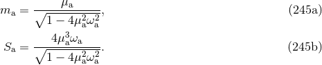
The total relativistic masses of the two Kerr black holes (with  labelling the black holes) are given
by54
labelling the black holes) are given
by54

 is the spin, related to the usual Kerr parameter by
  ,
and
,
and  is the irreducible mass, not to be confused with the reduced mass of the binary system, and
given by
is the irreducible mass, not to be confused with the reduced mass of the binary system, and
given by  (
( is the hole’s surface area). The angular velocity of the black hole, defined by
the angular velocity of the outgoing photons that remain for ever at the location of the light-like horizon, is
We shall give in Eq. (284) below a more general formulation of the “internal structure” of the black
holes. Combining Eqs. (243*) – (244*) we obtain
is the hole’s surface area). The angular velocity of the black hole, defined by
the angular velocity of the outgoing photons that remain for ever at the location of the light-like horizon, is
We shall give in Eq. (284) below a more general formulation of the “internal structure” of the black
holes. Combining Eqs. (243*) – (244*) we obtain 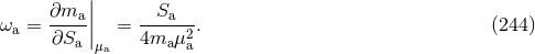
 and
and  as functions of
  and
and  ,
,
In the limit of slow rotation we get
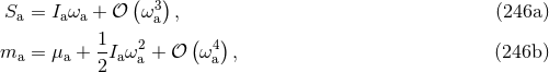
where  is the moment of inertia of the black hole. We see that the total mass-energy
  involves the irreducible mass augmented by the usual kinetic energy of the spin.
We now need the relation between the rotation frequency  of each of the corotating black
holes and the orbital frequency
of each of the corotating black
holes and the orbital frequency  of the binary system. Indeed
  is the basic variable
describing each equilibrium configuration calculated numerically in Refs. [232*, 133*], with the
irreducible masses held constant along the numerical evolutionary sequences. Here we report the
result of an investigation of the condition for corotation based on the first law of mechanics for
spinning black holes [55*], which concluded that the corotation condition at 2PN order reads
is the basic variable
describing each equilibrium configuration calculated numerically in Refs. [232*, 133*], with the
irreducible masses held constant along the numerical evolutionary sequences. Here we report the
result of an investigation of the condition for corotation based on the first law of mechanics for
spinning black holes [55*], which concluded that the corotation condition at 2PN order reads

 denotes the post-Newtonian parameter (230*) and
  the symmetric mass ratio
(215*). The condition (247*) is issued from the general relation which will be given in Eq. (285*).
Interestingly, notice that
the symmetric mass ratio
(215*). The condition (247*) is issued from the general relation which will be given in Eq. (285*).
Interestingly, notice that  up to the rather high 2PN order. In the Newtonian limit
 or the test-particle limit
  we simply have
  , in agreement with physical
intuition.
, in agreement with physical
intuition.
To take into account the spin effects our first task is to replace all the masses entering the
energy function (232) by their equivalent expressions in terms of  and the irreducible masses
 , and then to replace
  in terms of
  according to the corotation prescription
(247*).55
It is clear that the leading contribution is that of the spin kinetic energy given in Eq. (246b),
and it comes from the replacement of the rest mass-energy
according to the corotation prescription
(247*).55
It is clear that the leading contribution is that of the spin kinetic energy given in Eq. (246b),
and it comes from the replacement of the rest mass-energy  . From Eq. (246b)
this effect is of order
. From Eq. (246b)
this effect is of order  in the case of corotating binaries, which means by comparison with
Eq. (232) that it is equivalent to an “orbital” effect at the 2PN order (i.e.,
in the case of corotating binaries, which means by comparison with
Eq. (232) that it is equivalent to an “orbital” effect at the 2PN order (i.e.,  ). Higher-order
corrections in Eq. (246b), which behave at least like
). Higher-order
corrections in Eq. (246b), which behave at least like  , will correspond to the orbital 5PN order
at least and are negligible for the present purpose. In addition there will be a subdominant
contribution, of the order of
, will correspond to the orbital 5PN order
at least and are negligible for the present purpose. In addition there will be a subdominant
contribution, of the order of  equivalent to 3PN order, which comes from the replacement
of the masses into the Newtonian part, proportional to
equivalent to 3PN order, which comes from the replacement
of the masses into the Newtonian part, proportional to  , of the energy
  ; see
Eq. (232). With the 3PN accuracy we do not need to replace the masses that enter into the
post-Newtonian corrections in
; see
Eq. (232). With the 3PN accuracy we do not need to replace the masses that enter into the
post-Newtonian corrections in  , so in these terms the masses can be considered to be the irreducible
ones.
, so in these terms the masses can be considered to be the irreducible
ones.
Our second task is to include the specific relativistic effects due to the spins, namely the spin-orbit (SO)
interaction and the spin-spin (SS) one. In the case of spins  and
and  aligned parallel to the orbital
angular momentum (and right-handed with respect to the sense of motion) the SO energy reads
aligned parallel to the orbital
angular momentum (and right-handed with respect to the sense of motion) the SO energy reads
![[( ) ( ) ] 5∕3 4 m21 S1 4m22 S2 ESO = − m ν(m Ω) ----2 + ν --2 + ---2 + ν --2 . (248 ) 3 m m 1 3m m 2](article1908x.gif)

![[ ] ΔEcorot = μxμ (2 − 6η )x2 + η (− 10 + 25η )x3 + 𝒪 (x4) . (250 ) μ μ μ](article1911x.gif)
 , the symmetric mass ratio
  , and the dimensionless invariant
post-Newtonian parameter
, and the dimensionless invariant
post-Newtonian parameter  are now expressed in terms of the irreducible masses
  , rather
than the masses
, rather
than the masses  . The complete 3PN energy of the corotating binary is finally given by the sum of
Eqs. (232) and (250*), in which all the masses are now understood as being the irreducible ones, which must
be assumed to stay constant when the binary evolves for the comparison with the numerical
calculation.
. The complete 3PN energy of the corotating binary is finally given by the sum of
Eqs. (232) and (250*), in which all the masses are now understood as being the irreducible ones, which must
be assumed to stay constant when the binary evolves for the comparison with the numerical
calculation.
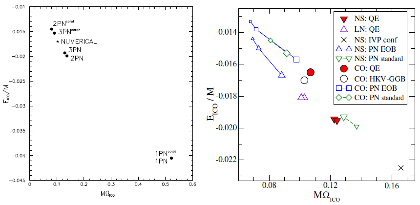
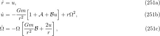
 versus
  in the equal-mass case (
 ). Left panel:
Comparison with the numerical relativity result of Gourgoulhon, Grandclément et al. [228*, 232*]
valid in the corotating case (marked by a star). Points indicated by
). Left panel:
Comparison with the numerical relativity result of Gourgoulhon, Grandclément et al. [228*, 232*]
valid in the corotating case (marked by a star). Points indicated by  are computed from the
minimum of Eq. (232), and correspond to irrotational binaries. Points denoted by
are computed from the
minimum of Eq. (232), and correspond to irrotational binaries. Points denoted by  come
from the minimum of the sum of Eqs. (232) and (250*), and describe corotational binaries. Note
the very good convergence of the standard (Taylor-expanded) PN series. Right panel: Numerical
relativity results of Cook, Pfeiffer et al. [133*, 121*] for quasi-equilibrium (QE) configurations and
various boundary conditions for the lapse function, in the non-spinning (NS), leading-order non
spinning (LN) and corotating (CO) cases. The point from [228*, 232*] (HKV-GGB) is also reported
as in the left panel, together with IVP, the initial value approach with effective potential [132*, 342*],
as well as standard PN predictions from the left panel and non-standard (EOB) ones. The agreement
between the QE computation and the standard non-resummed 3PN point is excellent especially in
the irrotational NS case.
come
from the minimum of the sum of Eqs. (232) and (250*), and describe corotational binaries. Note
the very good convergence of the standard (Taylor-expanded) PN series. Right panel: Numerical
relativity results of Cook, Pfeiffer et al. [133*, 121*] for quasi-equilibrium (QE) configurations and
various boundary conditions for the lapse function, in the non-spinning (NS), leading-order non
spinning (LN) and corotating (CO) cases. The point from [228*, 232*] (HKV-GGB) is also reported
as in the left panel, together with IVP, the initial value approach with effective potential [132*, 342*],
as well as standard PN predictions from the left panel and non-standard (EOB) ones. The agreement
between the QE computation and the standard non-resummed 3PN point is excellent especially in
the irrotational NS case. The left panel of Figure 1* shows the results for  in the case of irrotational and corotational
binaries. Since
in the case of irrotational and corotational
binaries. Since  , given by Eq. (250*), is at least of order 2PN, the result for
  is the same
as for 1PN in the irrotational case; then, obviously,
is the same
as for 1PN in the irrotational case; then, obviously,  takes into account only the leading 2PN
corotation effect, i.e., the spin kinetic energy given by Eq. (246b), while
takes into account only the leading 2PN
corotation effect, i.e., the spin kinetic energy given by Eq. (246b), while  involves also, in
particular, the corotational SO coupling at the 3PN order. In addition we present the numerical point
obtained by numerical relativity under the assumptions of conformal flatness and of helical
symmetry [228*, 232*]. As we can see the 3PN points, and even the 2PN ones, are in good agreement with
the numerical value. The fact that the 2PN and 3PN values are so close to each other is a good sign of the
convergence of the expansion. In fact one might say that the role of the 3PN approximation is merely to
“confirm” the value already given by the 2PN one (but of course, had we not computed the 3PN term, we
would not be able to trust very much the 2PN value). As expected, the best agreement we obtain is
for the 3PN approximation and in the case of corotation, i.e., the point
involves also, in
particular, the corotational SO coupling at the 3PN order. In addition we present the numerical point
obtained by numerical relativity under the assumptions of conformal flatness and of helical
symmetry [228*, 232*]. As we can see the 3PN points, and even the 2PN ones, are in good agreement with
the numerical value. The fact that the 2PN and 3PN values are so close to each other is a good sign of the
convergence of the expansion. In fact one might say that the role of the 3PN approximation is merely to
“confirm” the value already given by the 2PN one (but of course, had we not computed the 3PN term, we
would not be able to trust very much the 2PN value). As expected, the best agreement we obtain is
for the 3PN approximation and in the case of corotation, i.e., the point  . However,
the 1PN approximation is clearly not precise enough, but this is not surprising in the highly
relativistic regime of the ICO. The right panel of Figure 1* shows other very interesting comparisons
with numerical relativity computations [133*, 121*], done not only for the case of corotational
binaries but also in the irrotational (non-spinning) case. Witness in particular the almost perfect
agreement between the standard 3PN point (PN standard, shown with a green triangle) and the
numerical quasi-equilibrium point (QE, red triangle) in the case of irrotational non-spinning (NS)
binaries.
. However,
the 1PN approximation is clearly not precise enough, but this is not surprising in the highly
relativistic regime of the ICO. The right panel of Figure 1* shows other very interesting comparisons
with numerical relativity computations [133*, 121*], done not only for the case of corotational
binaries but also in the irrotational (non-spinning) case. Witness in particular the almost perfect
agreement between the standard 3PN point (PN standard, shown with a green triangle) and the
numerical quasi-equilibrium point (QE, red triangle) in the case of irrotational non-spinning (NS)
binaries.
However, we recall that the numerical works [228*, 232*, 133*, 121*] assume that the spatial metric is conformally flat, which is incompatible with the post-Newtonian approximation starting from the 2PN order (see [196] for a discussion). Nevertheless, the agreement found in Figure 1* constitutes an appreciable improvement of the previous situation, because the first estimations of the ICO in post-Newtonian theory [274] and numerical relativity [132, 342, 29] disagreed with each other, and do not match with the present 3PN results.
8.2 Dynamical stability of circular orbits
In this section, following Ref. [79*], we shall investigate the problem of the stability, against dynamical perturbations, of circular orbits at the 3PN order. We propose to use two different methods, one based on a linear perturbation at the level of the center-of-mass equations of motion (219*) – (220) in (standard) harmonic coordinates, the other one consisting of perturbing the Hamiltonian equations in ADM coordinates for the center-of-mass Hamiltonian (223). We shall find a criterion for the stability of circular orbits and shall present it in an invariant way – the same in different coordinate systems. We shall check that our two methods agree on the result.
We deal first with the perturbation of the equations of motion, following Kidder, Will & Wiseman [275*]
(see their Section III.A). We introduce polar coordinates  in the orbital plane and pose
  and
and
 . Then Eq. (219*) yields the system of equations
where  and
and  are given by Eqs. (220) as functions of
  ,
,  and
and  (through
 ).
).
In the case of an orbit that is circular apart from the adiabatic inspiral at the 2.5PN order (we neglect
the radiation-reaction damping effects), we have  hence
hence  . In this section we shall
indicate quantities associated with the circular orbit, which constitutes the zero-th approximation in our
perturbation scheme, using the subscript
. In this section we shall
indicate quantities associated with the circular orbit, which constitutes the zero-th approximation in our
perturbation scheme, using the subscript  . Hence Eq. (251b) gives the angular velocity
  of the
circular orbit as
of the
circular orbit as

 as a function of the circular-orbit radius
  in standard harmonic coordinates; the result agrees with
Eq. (228).57
in standard harmonic coordinates; the result agrees with
Eq. (228).57
We now investigate the linear perturbation around the circular orbit defined by the constants  ,
,
 and
and  . We pose
where  ,
,  and
and  denote the linear perturbations of the circular orbit. Then a system of linear
equations readily follows:
denote the linear perturbations of the circular orbit. Then a system of linear
equations readily follows:
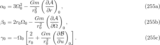
where the coefficients, which solely depend on the unperturbed circular orbit (hence the added subscript
 ), read as [275*]
In obtaining these equations we use the fact that  is a function of the square
  through
 , so that
  is proportional to
  and thus vanishes in the unperturbed
configuration (because
and thus vanishes in the unperturbed
configuration (because  ). On the other hand, since the radiation reaction is neglected,
  is also
proportional to
is also
proportional to  [see Eq. (220b)], so only
  can contribute at the zero-th perturbative order.
Now by examining the fate of perturbations that are proportional to some
can contribute at the zero-th perturbative order.
Now by examining the fate of perturbations that are proportional to some  , we arrive at the condition
for the frequency
, we arrive at the condition
for the frequency  of the perturbation to be real, and hence for stable circular orbits to exist, as being
[275*]
of the perturbation to be real, and hence for stable circular orbits to exist, as being
[275*]

 and
and  at the 3PN order we then arrive at the orbital-stability
criterion
at the 3PN order we then arrive at the orbital-stability
criterion
where we recall that  is the radius of the orbit in harmonic coordinates.
Our second method is to use the Hamiltonian equations associated with the 3PN center-of-mass
Hamiltonian in ADM coordinates  given by Eq. (223). We introduce the polar coordinates
  in the orbital plane – we assume that the orbital plane is equatorial, given by
  in the spherical
coordinate system
in the spherical
coordinate system  – and make the substitution

 ,
,  and
and  , and describes the motion in
polar coordinates in the orbital plane; henceforth we denote it by
, and describes the motion in
polar coordinates in the orbital plane; henceforth we denote it by ![ℋ = ℋ [R, PR, PΨ ] ≡ HADM ∕ μ](article1983x.gif) . The
Hamiltonian equations then read
. The
Hamiltonian equations then read
Evidently the constant  is nothing but the conserved angular-momentum integral. For circular
orbits we have
is nothing but the conserved angular-momentum integral. For circular
orbits we have  (a constant) and
  , so
, so
![∂ℋ-[ 0] ∂R R0, 0,PΨ = 0, (260 )](article1988x.gif)
 of the circular orbit as a function of
  , and
which yields the angular frequency of the circular orbit
, and
which yields the angular frequency of the circular orbit ![( d Ψ ) ∂ℋ [ ] Ω0 ≡ --- = ----- R0,0,P 0Ψ , (261 ) dt 0 ∂P Ψ](article1991x.gif)
 , which is evidently the same numerical
quantity as in Eq. (252*), but is here expressed in terms of the separation
, which is evidently the same numerical
quantity as in Eq. (252*), but is here expressed in terms of the separation  in ADM coordinates. The
last equation, which is equivalent to
in ADM coordinates. The
last equation, which is equivalent to  , is
It is automatically verified because
, is
It is automatically verified because ![-∂ℋ--[R0,0,P 0] = 0. (262 ) ∂PR Ψ](article1995x.gif)
 is a quadratic function of
  and hence
  is zero for
circular orbits.
is zero for
circular orbits.
We consider now a perturbation of the circular orbit defined by
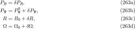
The Hamiltonian equations (259), worked out at the linearized order, read as
where the coefficients, which depend on the unperturbed orbit, are given by
By looking to solutions proportional to some  one obtains some real frequencies, and therefore one
finds stable circular orbits, if and only if
one obtains some real frequencies, and therefore one
finds stable circular orbits, if and only if

This result does not look the same as our previous result (257), but this is simply due to the fact that it
depends on the ADM radial separation  instead of the harmonic one
  . Fortunately we have derived
in Section 7.2 the material needed to connect
. Fortunately we have derived
in Section 7.2 the material needed to connect  to
to  with the 3PN accuracy. Indeed,
with Eqs. (210*) we have the relation valid for general orbits in an arbitrary frame between the
separation vectors in both coordinate systems. Specializing that relation to circular orbits we
find
with the 3PN accuracy. Indeed,
with Eqs. (210*) we have the relation valid for general orbits in an arbitrary frame between the
separation vectors in both coordinate systems. Specializing that relation to circular orbits we
find

Note that the difference between  and
and  starts only at 2PN order. That relation easily permits to
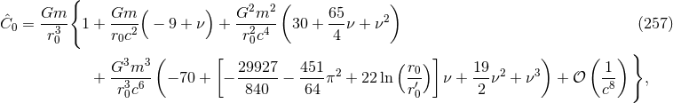
perfectly reconcile both expressions (257) and (267).
starts only at 2PN order. That relation easily permits to
perfectly reconcile both expressions (257) and (267).
Finally let us give to  an invariant meaning by expressing it with the help of the orbital frequency
 of the circular orbit, or, more conveniently, of the frequency-related parameter
  –
cf. Eq. (230*). This allows us to write the criterion for stability as
–
cf. Eq. (230*). This allows us to write the criterion for stability as  , where
 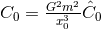 admits
the gauge-invariant form
admits
the gauge-invariant form
![( [ ] ) 2 397- 123- 2 2 3 ( 4) C0 = 1 − 6x0 + 14 νx0 + 2 − 16 π ν − 14ν x0 + 𝒪 x0 . (269 )](article2017x.gif)
 )
is located at
)
is located at  . Thus we find that, at the 1PN order, but for any mass ratio
  ,
One could have expected that some deviations of the order of
,
One could have expected that some deviations of the order of 
 already occur at the 1PN order, but it
turns out that only from the 2PN order does one find the occurrence of some non-Schwarzschildean
corrections proportional to
already occur at the 1PN order, but it
turns out that only from the 2PN order does one find the occurrence of some non-Schwarzschildean
corrections proportional to  . At the 2PN order we obtain
For equal masses this gives
. At the 2PN order we obtain
For equal masses this gives 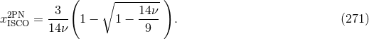
 . Notice also that the effect of the finite mass corrections is to
increase the frequency of the ISCO with respect to the Schwarzschild result, i.e., to make it more
inward:58
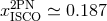
Finally, at the 3PN order, for equal masses
. Notice also that the effect of the finite mass corrections is to
increase the frequency of the ISCO with respect to the Schwarzschild result, i.e., to make it more
inward:58
Finally, at the 3PN order, for equal masses ![[ ] x2PN = 1-1 + 7-ν + 𝒪 (ν2) . (272 ) ISCO 6 18](article2026x.gif)
 , we find that according to our criterion all the circular
orbits are stable. More generally, we find that at the 3PN order all orbits are stable when the mass ratio
, we find that according to our criterion all the circular
orbits are stable. More generally, we find that at the 3PN order all orbits are stable when the mass ratio  is larger than some critical value
  .
.
The stability criterion (269*) has been compared in great details to various other stability criteria by Favata [191*] and shown to perform very well, and has also been generalized to spinning black hole binaries in Ref. [190]. Note that this criterion is based on the physical requirement that a stable perturbation should have a real frequency. It gives an innermost stable circular orbit, when it exists, which differs from the innermost circular orbit or ICO defined in Section 8.1; see Ref. [378] for a discussion on the difference between an ISCO and the ICO in the PN context. Note also that the criterion (269*) is based on systematic post-Newtonian expansions, without resorting for instance to Padé approximants. Nevertheless, it performs better than other criteria based on various resummation techniques, as discussed in Ref. [191].
8.3 The first law of binary point-particle mechanics
In this section we shall review a very interesting relation for binary systems of point particles modelling black hole binaries and moving on circular orbits, known as the “first law of point-particle mechanics”. This law was obtained using post-Newtonian methods in Ref. [289*], but is actually a particular case of a more general law, valid for systems of black holes and extended fluid balls, derived by Friedman, Uryū & Shibata [208*].
Before tackling the problem it is necessary to make more precise the notion of circular orbits. These are obtained from the conservative part of the dynamics, neglecting the dissipative radiation-reaction force responsible for the gravitational-wave inspiral. In post-Newtonian theory this means neglecting the radiation-reaction force at 2.5PN and 3.5PN orders, i.e., considering only the conservative dynamics at the even-parity 1PN, 2PN and 3PN orders. We have seen in Sections 5.2 and 5.4 that this clean separation between conservative even-parity and dissipative odd-parity terms breaks at 4PN order, because of a contribution originating from gravitational-wave tails in the radiation-reaction force. We expect that at any higher order 4PN, 4.5PN, 5PN, etc. there will be a mixture of conservative and dissipative effects; here we assume that at any higher order we can neglect the radiation-reaction dissipation effects.
Consider a system of two compact objects moving on circular orbits. We examine first the case of
non-spinning objects. With exactly circular orbits the geometry admits a helical Killing vector (HKV) field
 , satisfying the Killing equation
  . Imposing the existence of the HKV is the
rigorous way to implement the notion of circular orbits. A Killing vector is only defined up to an overall
constant factor. The helical Killing vector
. Imposing the existence of the HKV is the
rigorous way to implement the notion of circular orbits. A Killing vector is only defined up to an overall
constant factor. The helical Killing vector  extends out to a large distance where the geometry is
essentially flat. There,
extends out to a large distance where the geometry is
essentially flat. There,

 denotes the
angular frequency of the binary’s circular motion.
denotes the
angular frequency of the binary’s circular motion.
An observer moving with one of the particles (say the particle 1), while orbiting around the other
particle, would detect no change in the local geometry. Thus the four-velocity  of that particle is
tangent to the Killing vector
of that particle is
tangent to the Killing vector  evaluated at the location of the particle, which we denote by
  . A
physical quantity is then defined as the constant of proportionality
. A
physical quantity is then defined as the constant of proportionality  between these two vectors, namely

 , where
  denotes the metric at
the location of the particle. For a self-gravitating compact binary system, the metric at point 1 is generated
by the two particles and has to be regularized according to one of the self-field regularizations discussed in
Section 6. It will in fact be sometimes more convenient to work with the inverse of
denotes the metric at
the location of the particle. For a self-gravitating compact binary system, the metric at point 1 is generated
by the two particles and has to be regularized according to one of the self-field regularizations discussed in
Section 6. It will in fact be sometimes more convenient to work with the inverse of  , denoted
 . From Eq. (274*) we get
where
. From Eq. (274*) we get
where 
 denotes the usual space-time dot product. Thus we can regard
  as the
Killing energy of the particle that is associated with the HKV field
as the
Killing energy of the particle that is associated with the HKV field  . The quantity
  represents also
the redshift of light rays emitted from the particle and received on the helical symmetry axis perpendicular
to the orbital plane at large distances from it [176*]. In the following we shall refer to
represents also
the redshift of light rays emitted from the particle and received on the helical symmetry axis perpendicular
to the orbital plane at large distances from it [176*]. In the following we shall refer to  as the redshift
observable.
as the redshift
observable.
If we choose a coordinate system such that Eq. (273*) is satisfied everywhere, then in particular
 , thus
  simply agrees with
  , the
, the  -component of the four-velocity of the particle. The
Killing vector on the particle is then
-component of the four-velocity of the particle. The
Killing vector on the particle is then  , and simply reduces to the particle’s ordinary
coordinate velocity:
, and simply reduces to the particle’s ordinary
coordinate velocity:  where
where  and
and ![α y1(t) = [ct,y1(t)]](article2057x.gif) denotes the
particle’s trajectory in that coordinate system. The redshift observable we are thus considering is
denotes the
particle’s trajectory in that coordinate system. The redshift observable we are thus considering is

 , it does
not depend upon the choice of perturbative gauge with respect to the background metric. We shall be
interested in the invariant scalar function
, it does
not depend upon the choice of perturbative gauge with respect to the background metric. We shall be
interested in the invariant scalar function  , where
  is the angular frequency of the circular orbit
introduced when imposing Eq. (273*).
is the angular frequency of the circular orbit
introduced when imposing Eq. (273*).
We have obtained in Section 7.4 the expressions of the post-Newtonian binding energy  and angular
momentum
and angular
momentum  for point-particle binaries on circular orbits. We shall now show that there are some
differential and algebraic relations linking
for point-particle binaries on circular orbits. We shall now show that there are some
differential and algebraic relations linking  and
and  to the redshift observables
  and
and  associated
with the two individual particles. Here we prefer to introduce instead of
associated
with the two individual particles. Here we prefer to introduce instead of  the total relativistic (ADM)
mass of the binary system
the total relativistic (ADM)
mass of the binary system

 is the sum of the two post-Newtonian individual masses
  and
and  – those which have
been used up to now, for instance in Eq. (203). Note that in the spinning case such post-Newtonian masses
acquire some spin contributions given, e.g., by Eqs. (243*) – (246).
– those which have
been used up to now, for instance in Eq. (203). Note that in the spinning case such post-Newtonian masses
acquire some spin contributions given, e.g., by Eqs. (243*) – (246).
For point particles without spins, the ADM mass  , angular momentum
  , and redshifts
  , are
functions of three independent variables, namely the orbital frequency
, are
functions of three independent variables, namely the orbital frequency  that is imposed by the existence
of the HKV, and the individual masses
that is imposed by the existence
of the HKV, and the individual masses  . For spinning point particles, we have also the
two spins
. For spinning point particles, we have also the
two spins  which are necessarily aligned with the orbital angular momentum. We first
recover that the ADM quantities obey the “thermodynamical” relation already met in Eq. (235*),
which are necessarily aligned with the orbital angular momentum. We first
recover that the ADM quantities obey the “thermodynamical” relation already met in Eq. (235*),

 being the coefficient of proportionality. This relation is used in computations of the binary evolution
based on a sequence of quasi-equilibrium configurations [228, 232, 133, 121], as discussed in
Section 8.1.
being the coefficient of proportionality. This relation is used in computations of the binary evolution
based on a sequence of quasi-equilibrium configurations [228, 232, 133, 121], as discussed in
Section 8.1.
The first law will be a thermodynamical generalization of Eq. (278*), describing the changes in the ADM
quantities not only when the orbital frequency  varies with fixed masses, but also when the individual
masses
varies with fixed masses, but also when the individual
masses  of the particles vary with fixed orbital frequency. That is, one compares together different
conservative dynamics with different masses but the same frequency. This situation is answered by the
differential equations
of the particles vary with fixed orbital frequency. That is, one compares together different
conservative dynamics with different masses but the same frequency. This situation is answered by the
differential equations

Theorem 11. The changes in the ADM mass and angular momentum of a binary system made of point particles in response to infinitesimal variations of the individual masses of the point particles, are related together by the first law of binary point-particle mechanics as [208*, 289*]

This law was proved in a very general way in Ref. [208*] for systems of black holes and extended bodies under some arbitrary Killing symmetry. The particular form given in Eq. (280*) is a specialization to the case of point particle binaries with helical Killing symmetry. It has been proved directly in this form in Ref. [289*] up to high post-Newtonian order, namely 3PN order plus the logarithmic contributions occurring at 4PN and 5PN orders.
The first law of binary point-particle mechanics (280*) is of course reminiscent of the celebrated first law
of black hole mechanics  , which holds for any non-singular, asymptotically flat
perturbation of a stationary and axisymmetric black hole of mass
, which holds for any non-singular, asymptotically flat
perturbation of a stationary and axisymmetric black hole of mass  , intrinsic angular momentum (or
spin)
, intrinsic angular momentum (or
spin)  , surface area
  , uniform surface gravity
  , and angular frequency
  on the
horizon [26, 417]; see Ref. [289*] for a discussion.
on the
horizon [26, 417]; see Ref. [289*] for a discussion.
An interesting by-product of the first law (280*) is the remarkably simple algebraic relation
which can be seen as a first integral of the differential relation (280*). Note that the existence of such a simple algebraic relation between the local quantities
 and
and  on one hand, and the globally defined
quantities
on one hand, and the globally defined
quantities  and
and  on the other hand, is not trivial.
Next, we report the result of a generalization of the first law applicable to systems of point particles with spins (moving on
circular orbits).59
This result is valid through linear order in the spin of each particle, but holds also for the quadratic
coupling between different spins (interaction spin terms  in the language of Section 11). To be
consistent with the HKV symmetry, we must assume that the two spins
in the language of Section 11). To be
consistent with the HKV symmetry, we must assume that the two spins  are aligned or anti-aligned
with the orbital angular momentum. We introduce the total (ADM-like) angular momentum
are aligned or anti-aligned
with the orbital angular momentum. We introduce the total (ADM-like) angular momentum  which is
related to the orbital angular momentum
which is
related to the orbital angular momentum  by
by  for aligned or anti-aligned spins. The
first law now becomes [55*]
for aligned or anti-aligned spins. The
first law now becomes [55*]
![∑ [ ( ) ] δM − ΩδJ = zaδma + Ωa − Ω δSa , (282 ) a](article2101x.gif)
 denotes the precession frequency of the spins. This law has been derived in Ref. [55*]
from the canonical Hamiltonian formalism. The spin variables used here are the canonical spins
denotes the precession frequency of the spins. This law has been derived in Ref. [55*]
from the canonical Hamiltonian formalism. The spin variables used here are the canonical spins  ,
that are easily seen to obey, from the algebra satisfied by the canonical variables, the usual
Newtonian-looking precession equations
,
that are easily seen to obey, from the algebra satisfied by the canonical variables, the usual
Newtonian-looking precession equations  . These variables are identical to
the “constant-in-magnitude” spins which will be defined and extensively used in Section 11.
Similarly, to Eq. (281*) we have also a first integral associated with the variational law (282*):
. These variables are identical to
the “constant-in-magnitude” spins which will be defined and extensively used in Section 11.
Similarly, to Eq. (281*) we have also a first integral associated with the variational law (282*):
![∑ [ ] M − 2ΩJ = zama − 2(Ω − Ωa )Sa . (283 ) a](article2105x.gif)
Notice that the relation (282*) has been derived for point particles and arbitrary aligned spins. We would like now to derive the analogous relation for binary black holes. The key difference is that black holes are extended finite-size objects while point particles have by definition no spatial extension. For point particle binaries the spins can have arbitrary magnitude and still be compatible with the HKV. In this case the law (282*) would describe also (super-extremal) naked singularities. For black hole binaries the HKV constraints the rotational state of each black hole and the binary system must be corotating.
Let us derive, in a heuristic way, the analogue of the first law (282*) for black holes by introducing some
“constitutive relations”  specifying the energy content of the bodies, i.e., the relations
linking their masses
specifying the energy content of the bodies, i.e., the relations
linking their masses  to the spins
  and to some irreducible masses
  . More precisely, we define
for each spinning particle the analogue of an irreducible mass
. More precisely, we define
for each spinning particle the analogue of an irreducible mass  via the variational relation
 ,60
in which the “response coefficient”
,60
in which the “response coefficient”  of the body and its proper rotation frequency
  are associated
with the internal structure:
are associated
with the internal structure:
For instance, using the Christodoulou mass formula (243*) for Kerr black holes, we obtain the rotation
frequency  given by Eq. (244*). On the other hand, the response coefficient
  differs from 1 only
because of spin effects, and we can check that
differs from 1 only
because of spin effects, and we can check that  .
.
Within the latter heuristic model a condition for the corotation of black hole binaries has been proposed in Ref. [55] as
This condition determines the value of the proper frequency
 of each black hole appropriate to the
corotation state. When expanded to 2PN order the condition (285*) leads to Eq. (247*) that we have
already used in Section 8.1. With Eq. (285*) imposed, the first law (282*) simplifies considerably:
This is almost identical to the first law for non-spinning binaries given by Eq. (280*); indeed it simply differs
from it by the substitutions
of each black hole appropriate to the
corotation state. When expanded to 2PN order the condition (285*) leads to Eq. (247*) that we have
already used in Section 8.1. With Eq. (285*) imposed, the first law (282*) simplifies considerably:
This is almost identical to the first law for non-spinning binaries given by Eq. (280*); indeed it simply differs
from it by the substitutions 
 and
and  . Since the irreducible mass
  of a rotating black
hole is the spin-independent part of its total mass
of a rotating black
hole is the spin-independent part of its total mass  , this observation suggests that corotating binaries
are very similar to non-spinning binaries, at least from the perspective of the first law. Finally we can easily
reconcile the first law (286*) for corotating systems with the known first law of binary black hole
mechanics [208], namely
Indeed it suffices to make the formal identification in Eq. (286*) of
, this observation suggests that corotating binaries
are very similar to non-spinning binaries, at least from the perspective of the first law. Finally we can easily
reconcile the first law (286*) for corotating systems with the known first law of binary black hole
mechanics [208], namely
Indeed it suffices to make the formal identification in Eq. (286*) of 
 with
with  , where
  denotes
the constant surface gravity, and using the surface areas
denotes
the constant surface gravity, and using the surface areas  instead of the irreducible masses of
the black holes. This shows that the heuristic model based on the constitutive relations (284) is able to
capture the physics of corotating black hole binary systems.
instead of the irreducible masses of
the black holes. This shows that the heuristic model based on the constitutive relations (284) is able to
capture the physics of corotating black hole binary systems.
8.4 Post-Newtonian approximation versus gravitational self-force
The high-accuracy predictions from general relativity we have drawn up to now are well suited to describe
the inspiralling phase of compact binaries, when the post-Newtonian parameter (1*) is small
independently of the mass ratio  between the compact bodies. In this section we
investigate how well does the post-Newtonian expansion compare with another very important
approximation scheme in general relativity: The gravitational self-force approach, based on black-hole
perturbation theory, which gives an accurate description of extreme mass ratio binaries having
between the compact bodies. In this section we
investigate how well does the post-Newtonian expansion compare with another very important
approximation scheme in general relativity: The gravitational self-force approach, based on black-hole
perturbation theory, which gives an accurate description of extreme mass ratio binaries having
 or equivalently
  , even in the strong field regime. The gravitational self-force
analysis [317, 360, 178*, 231] (see [348, 177, 23] for reviews) is thus expected to provide templates for
extreme mass ratio inspirals (EMRI) anticipated to be present in the bandwidth of space-based
detectors.
, even in the strong field regime. The gravitational self-force
analysis [317, 360, 178*, 231] (see [348, 177, 23] for reviews) is thus expected to provide templates for
extreme mass ratio inspirals (EMRI) anticipated to be present in the bandwidth of space-based
detectors.
Consider a system of two (non-spinning) compact objects with 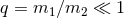 ; we shall call the
smaller mass
; we shall call the
smaller mass  the “particle”, and the larger mass
  the “black hole”. The orbit of the particle
around the black hole is supposed to be exactly circular as we neglect the radiation-reaction effects. With
circular orbits and no dissipation, we are considering the conservative part of the dynamics, and the
geometry admits the HKV field (273*). Note that in self-force theory there is a clean split between the
dissipative and conservative parts of the dynamics (see e.g., [22]). This split is particularly transparent for
an exact circular orbit, since the radial component (along
the “black hole”. The orbit of the particle
around the black hole is supposed to be exactly circular as we neglect the radiation-reaction effects. With
circular orbits and no dissipation, we are considering the conservative part of the dynamics, and the
geometry admits the HKV field (273*). Note that in self-force theory there is a clean split between the
dissipative and conservative parts of the dynamics (see e.g., [22]). This split is particularly transparent for
an exact circular orbit, since the radial component (along  ) is the only non-vanishing component of the
conservative self-force, while the dissipative part of the self-force are the components along
) is the only non-vanishing component of the
conservative self-force, while the dissipative part of the self-force are the components along  and
and
 .
.
 and the post-Newtonian parameter
 . Post-Newtonian theory and perturbative self-force analysis can be
compared in the post-Newtonian regime (
. Post-Newtonian theory and perturbative self-force analysis can be
compared in the post-Newtonian regime ( thus
thus  ) of an extreme mass ratio
(
) of an extreme mass ratio
( ) binary.
 The problem of the comparison between the post-Newtonian and perturbative self-force analyses in their
common domain of validity, that of the slow-motion and weak-field regime of an extreme mass ratio binary,
is illustrated in Figure 2*. This problem has been tackled by Detweiler [176*], who computed numerically
within the self-force (SF) approach the redshift observable  associated with the particle, and compared
it with the 2PN prediction extracted from existing post-Newtonian results [76]. This comparison proved to
be successful, and was later systematically implemented and extended to higher post-Newtonian orders
in Refs. [68*, 67*]. In this section we review the works [68*, 67*] which have demonstrated an
excellent agreement between the analytical post-Newtonian result derived through 3PN order, with
inclusion of specific logarithmic terms at 4PN and 5PN orders, and the exact numerical SF
result.
associated with the particle, and compared
it with the 2PN prediction extracted from existing post-Newtonian results [76]. This comparison proved to
be successful, and was later systematically implemented and extended to higher post-Newtonian orders
in Refs. [68*, 67*]. In this section we review the works [68*, 67*] which have demonstrated an
excellent agreement between the analytical post-Newtonian result derived through 3PN order, with
inclusion of specific logarithmic terms at 4PN and 5PN orders, and the exact numerical SF
result.
For the PN-SF comparison, we require two physical quantities which are precisely defined in the context
of each of the approximation schemes. The orbital frequency  of the circular orbit as measured by a
distant observer is one such quantity and has been introduced in Eq. (273*); the second quantity is the
redshift observable
of the circular orbit as measured by a
distant observer is one such quantity and has been introduced in Eq. (273*); the second quantity is the
redshift observable  (or equivalently
  ) associated with the smaller mass
  and
defined by Eqs. (274*) or (275*). The truly coordinate and perturbative-gauge independent properties of
and
defined by Eqs. (274*) or (275*). The truly coordinate and perturbative-gauge independent properties of  and the redshift observable
  play a crucial role in this comparison. In the perturbative self-force
approach we use Schwarzschild coordinates for the background, and we refer to “gauge invariance” as a
property which holds within the restricted class of gauges for which (273*) is a helical Killing
vector. In all other respects, the gauge choice is arbitrary. In the post-Newtonian approach
we work with harmonic coordinates and compute the explicit expression (276*) of the redshift
observable.
play a crucial role in this comparison. In the perturbative self-force
approach we use Schwarzschild coordinates for the background, and we refer to “gauge invariance” as a
property which holds within the restricted class of gauges for which (273*) is a helical Killing
vector. In all other respects, the gauge choice is arbitrary. In the post-Newtonian approach
we work with harmonic coordinates and compute the explicit expression (276*) of the redshift
observable.
The main difficulty in the post-Newtonian calculation is the control to high PN order of the near-zone
metric  entering the definition of the redshift observable (276*), and which has to be regularized at
the location of the particle by means of dimensional regularization (see Sections 6.3 – 6.4). Up to 2.5PN
order the Hadamard regularization is sufficient and the regularized metric has been provided in Eqs. (242).
Here we report the end result of the post-Newtonian computation of the redshift observable including all
terms up to the 3PN order, and augmented by the logarithmic contributions up to the 5PN order (and also
the known Schwarzschild limit) [68*, 67*, 289*]:
entering the definition of the redshift observable (276*), and which has to be regularized at
the location of the particle by means of dimensional regularization (see Sections 6.3 – 6.4). Up to 2.5PN
order the Hadamard regularization is sufficient and the regularized metric has been provided in Eqs. (242).
Here we report the end result of the post-Newtonian computation of the redshift observable including all
terms up to the 3PN order, and augmented by the logarithmic contributions up to the 5PN order (and also
the known Schwarzschild limit) [68*, 67*, 289*]:
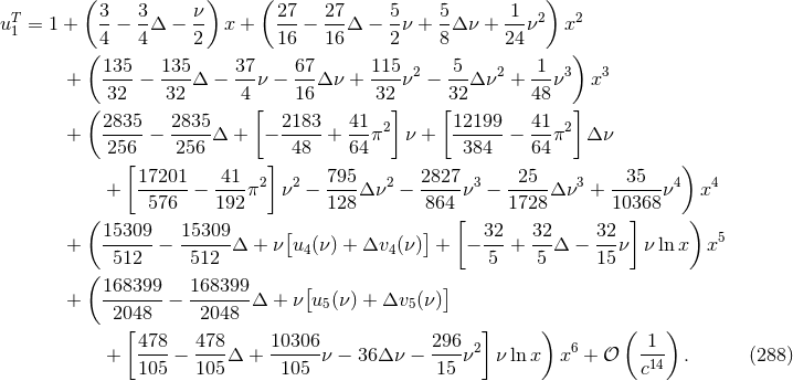
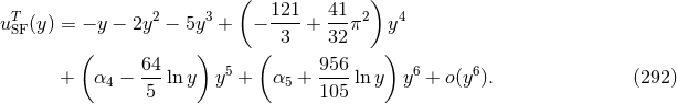
We recall that  denotes the post-Newtonian parameter (230*),
  is the mass ratio (215*),
and
is the mass ratio (215*),
and  . The redshift observable of the other particle is deduced by setting
 .
.
In Eq. (288) we denote by  ,
,  and
and  ,
,  some unknown 4PN and
5PN coefficients, which are however polynomials of the symmetric mass ratio
some unknown 4PN and
5PN coefficients, which are however polynomials of the symmetric mass ratio  . They can
be entirely determined from the related coefficients
. They can
be entirely determined from the related coefficients  ,
,  and
and  ,
,  in
the expressions of the energy and angular momentum in Eqs. (233) and (234). To this aim
it suffices to apply the differential first law (280*) up to 5PN order; see Ref. [289] for more
details.
in
the expressions of the energy and angular momentum in Eqs. (233) and (234). To this aim
it suffices to apply the differential first law (280*) up to 5PN order; see Ref. [289] for more
details.
The post-Newtonian result (288) is valid for any mass ratio, and for comparison purpose with the SF
calculation we now investigate the small mass ratio regime  . We introduce a post-Newtonian
parameter appropriate to the small mass limit of the “particle”,
. We introduce a post-Newtonian
parameter appropriate to the small mass limit of the “particle”,

 , together with
 . Then Eq. (288), expanded through first order in
  , which means including only
the linear self-force level, reads
The Schwarzschildean result is known in closed form as
and for the self-force contribution one
obtains61
, which means including only
the linear self-force level, reads
The Schwarzschildean result is known in closed form as
and for the self-force contribution one
obtains61


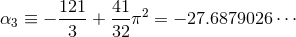
The analytic coefficients were determined up to 2PN order in Ref. [176*]; the 3PN term was computed in Ref. [68*] making full use of dimensional regularization; the logarithmic contributions at the 4PN and 5PN orders were added in Refs. [67*, 146].
The coefficients  and
and  represent some pure numbers at the 4PN and 5PN orders. By an analytic
self-force calculation [36] the coefficient
represent some pure numbers at the 4PN and 5PN orders. By an analytic
self-force calculation [36] the coefficient  has been obtained as

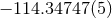
On the self-force front the main problem is to control the numerical resolution of the computation of the redshift observable in order to distinguish more accurately the contributions of very high order PN terms. The comparison of the post-Newtonian expansion (292) with the numerical SF data has confirmed with high precision the determination of the 3PN coefficient [68*, 67*]: Witness Table 1 where the agreement with the analytical value involves 7 significant digits. Notice that such agreement provides an independent check of the dimensional regularization procedure invoked in the PN expansion scheme (see Sections 6.3 – 6.4). It is remarkable that such procedure is equivalent to the procedure of subtraction of the singular field in the SF approach [178].
| 3PN coefficient | SF value |
 |
 |
| PN coefficient | SF value |
 |
 |
 |
 |
 |
 |
 |
 |
 |
 |
Furthermore the PN-SF comparison has permitted to measure the coefficients  and
and  with at least 8 significant digits for the 4PN coefficient, and 5 significant digits for the 5PN
one. In Table 2 we report the result of the analysis performed in Refs. [68*, 67*] by making
maximum use of the analytical coefficients available at the time, i.e., all the coefficients up to
3PN order plus the logarithmic contributions at 4PN and 5PN orders. One uses a set of five
basis functions corresponding to the unknown non-logarithmic 4PN and 5PN coefficients
with at least 8 significant digits for the 4PN coefficient, and 5 significant digits for the 5PN
one. In Table 2 we report the result of the analysis performed in Refs. [68*, 67*] by making
maximum use of the analytical coefficients available at the time, i.e., all the coefficients up to
3PN order plus the logarithmic contributions at 4PN and 5PN orders. One uses a set of five
basis functions corresponding to the unknown non-logarithmic 4PN and 5PN coefficients  ,
,
 in Eq. (292), and augmented by the 6PN and 7PN non-logarithmic coefficients
  ,
,
 plus a coefficient
  for the logarithm at 6PN. A contribution
  from a logarithm at
7PN order is likely to confound with the
from a logarithm at
7PN order is likely to confound with the  coefficient. There is also the possibility of the
contribution of a logarithmic squared at 7PN order, but such a small effect is not permitted in this
fit.
coefficient. There is also the possibility of the
contribution of a logarithmic squared at 7PN order, but such a small effect is not permitted in this
fit.
Gladly we discover that the more recent analytical value of the 4PN coefficient, Eq. (293*), matches the numerical value which was earlier measured in Ref. [67*] (see Table 2). This highlights the predictive power of perturbative self-force calculations in determining numerically new post-Newtonian coefficients [176, 68, 67]. This ability is obviously due to the fact (illustrated in Figure 2*) that perturbation theory is legitimate in the strong field regime of the coalescence of black hole binary systems, which is inaccessible to the post-Newtonian method. Of course, the limitation of the self-force approach is the small mass-ratio limit; in this respect it is taken over by the post-Newtonian approximation.
More recently, the accuracy of the numerical computation of the self-force, and the comparison with the
post-Newtonian expansion, have been drastically improved by Shah, Friedman & Whiting [383*]. The PN
coefficients of the redshift observable were obtained to very high 10.5PN order both numerically and also
analytically, for a subset of coefficients that are either rational or made of the product of  with a
rational. The analytical values of the coefficients up to 6PN order have also been obtained from an
alternative self-force calculation [38*, 37*]. An interesting feature of the post-Newtonian expansion at high
order is the appearance of half-integral PN coefficients (i.e., of the type
with a
rational. The analytical values of the coefficients up to 6PN order have also been obtained from an
alternative self-force calculation [38*, 37*]. An interesting feature of the post-Newtonian expansion at high
order is the appearance of half-integral PN coefficients (i.e., of the type  PN where
  is an odd integer)
in the conservative dynamics of binary point particles, moving on exactly circular orbits. This is interesting
because any instantaneous (non-tail) term at any half-integral PN order will be zero for circular orbits, as
can be shown by a simple dimensional argument [77*]. Therefore half-integral coefficients can
appear only due to truly hereditary (tail) integrals. Using standard post-Newtonian methods
it has been proved in Refs. [77, 78] that the dominant half-integral PN term in the redshift
observable (292) occurs at the 5.5PN order (confirming the earlier finding of Ref. [383*]) and
originates from the non-linear “tail-of-tail” integrals investigated in Section 3.2. The results for the
5.5PN coefficient in Eq. (292), and also for the next-to-leading 6.5PN and 7.5PN ones, are
is an odd integer)
in the conservative dynamics of binary point particles, moving on exactly circular orbits. This is interesting
because any instantaneous (non-tail) term at any half-integral PN order will be zero for circular orbits, as
can be shown by a simple dimensional argument [77*]. Therefore half-integral coefficients can
appear only due to truly hereditary (tail) integrals. Using standard post-Newtonian methods
it has been proved in Refs. [77, 78] that the dominant half-integral PN term in the redshift
observable (292) occurs at the 5.5PN order (confirming the earlier finding of Ref. [383*]) and
originates from the non-linear “tail-of-tail” integrals investigated in Section 3.2. The results for the
5.5PN coefficient in Eq. (292), and also for the next-to-leading 6.5PN and 7.5PN ones, are

To conclude, the consistency of this “cross-cultural” comparison between the analytical post-Newtonian and the perturbative self-force approaches confirms the soundness of both approximations in describing the dynamics of compact binaries. Furthermore this interplay between PN and SF efforts (which is now rapidly growing [383]) is important for the synthesis of template waveforms of EMRIs to be analysed by space-based gravitational wave detectors, and has also an impact on efforts of numerical relativity in the case of comparable masses.
 |
 |
 |