3 Interlude: Meanderings – UFT in the late 1930s and the 1940s
Prior to a discussion of the main research groups concerned with Einstein–Schrödinger theories, some approaches using the ideas of Kaluza and Klein for a unified field theory, or aspiring to bind together quantum theory and gravitation are discussed.
3.1 Projective and conformal relativity theory
Projective relativity theory had been invented expressly in order to avoid the fifth dimension of
Kaluza–Klein theory. In Sections 6.3.2 and 7.2.4 of Part I, Pauli & Solomon’s paper was described. Also, in
Section 6.3.2 of Part I, we briefly have discussed what O. Veblen & B. Hoffmann called “projective
relativity” [671*], and the relationship to the Einstein–Mayer theory. Veblen & Hoffmann had introduced
projective tensors with components  where
where  are
coordinates of space-time,
are
coordinates of space-time,  is an additional parameter (a gauge variable) and
  a constant named
“index”.40
a constant named
“index”.40
 transforms as
  . The auxiliary 5-dimensional space appearing has no physical
significance. A projective symmetric metric
. The auxiliary 5-dimensional space appearing has no physical
significance. A projective symmetric metric  of index
  was given by
  where
where  is
an arbitrary projective scalar of index
is
an arbitrary projective scalar of index  . In addition, a third symmetric tensor
  , the
gravitational metric, appeared. Here,
, the
gravitational metric, appeared. Here,  is a projective vector. Likewise, the Levi-Civita
connections
is a projective vector. Likewise, the Levi-Civita
connections  with
with  with
with  and
and
 were used. For arbitrary index
  , the field equations were derived from the curvature
scalar
, the field equations were derived from the curvature
scalar  calculated from the connection
  . One equation could be written in the form of a
wave equation:
. One equation could be written in the form of a
wave equation:

 is the curvature scalar calculated from
  . Veblen & Hoffmann concluded that: “The use of
projective tensors and projective geometry in relativity theory therefore seems to make it possible to bring
wave mechanics into the relativity scheme” ([671], abstract). How Planck’s constant might be brought in, is
left in the dark.
. Veblen & Hoffmann concluded that: “The use of
projective tensors and projective geometry in relativity theory therefore seems to make it possible to bring
wave mechanics into the relativity scheme” ([671], abstract). How Planck’s constant might be brought in, is
left in the dark.
During the 1940s, meson physics became fashionable. Of course, the overwhelming amount of this research happened in connection with nuclear and elementary particle theory, outside of UFT, but sometimes also in classical field theory. Cf. the papers by F. J. Belinfante on the meson field, in which he used the undor-formalism41 [16, 15]. In his doctoral thesis of 1941, “Projective theory of meson fields and electromagnetic properties of atomic nuclei” suggested by L. Rosenfeld, Abraham Pais in Utrecht kept away from UFT and calculated the projective energy momentum tensor of an arbitrary field. Although citing the paper of Veblen and Hoffmann, in projective theory he followed the formalism of Pauli; in his application to the Dirac spinor-field, he used Belinfantes undors [466]. After this paper, he examined which of Kemmer’s five types of meson fields were “in accordance with the requirements of projective relativity” ([467], p. 268).
It is unsurprising that B. Hoffmann in Princeton also applied the projective formalism to
a theory intended to unify the gravitational and vector meson fields [278*]. The meson field
 was defined by Hoffmann via:
  with
with  and
and  given above. Its
space-time components
given above. Its
space-time components  form an affine vector from which the vector meson field tensor
 follows. The theory again contained three Riemannian curvature tensors
(scalars). By skipping all calculations, we arrive at the affine form of Hoffmann’s field equations
follows. The theory again contained three Riemannian curvature tensors
(scalars). By skipping all calculations, we arrive at the affine form of Hoffmann’s field equations

 , these are the classical (i.e. unquantized) field
equations for a vector meson and gravitational field in the general theory of relativity” ([278], p. 464). We
could name them as well “Einstein-meson” equations in analogy to “Einstein–Maxwell” equations: no
unification of both field had been reached. Also, no scalar meson field and the electromagnetic field were
present in the theory.
, these are the classical (i.e. unquantized) field
equations for a vector meson and gravitational field in the general theory of relativity” ([278], p. 464). We
could name them as well “Einstein-meson” equations in analogy to “Einstein–Maxwell” equations: no
unification of both field had been reached. Also, no scalar meson field and the electromagnetic field were
present in the theory.
Hoffmann then looked for a “broader geometrical base” than projective geometry in order to include the
electromagnetic field. He found it in conformal geometry, or rather in a special subcase, similarity geometry
[279].42
It turned out that a 6-dimensional auxiliary space was needed. We shall denote the coordinates in this  by
by  . The components of a similarity tensor are
  ,
where
,
where  are the number of covariant and contravariant coordinate indices while
  again is
named the index of the tensor. In place of the transformations in projective geometry, now
again is
named the index of the tensor. In place of the transformations in projective geometry, now

 in
in  was given the role of metric; the assumptions
  and
and  independent of
  reduced the number of free functions. The definitions
  and
and
 led back to the former vector meson field via
  and to
a vector in
and to
a vector in 
 with
with  ,
,  independent of
  and containing the
electromagnetic 4-vector
and containing the
electromagnetic 4-vector  . To abreviate the story, Hoffmann’s final field equations in space-time were:
The last equation with
. To abreviate the story, Hoffmann’s final field equations in space-time were:
The last equation with 
 reproduced Maxwell’s equations. In a sequel to this paper,
Hoffmann claimed to have derived “the correct trajectories of charged meson testparticles in a combined
gravitational, electromagnetic, and vector meson field” ([280], p. 1045).
reproduced Maxwell’s equations. In a sequel to this paper,
Hoffmann claimed to have derived “the correct trajectories of charged meson testparticles in a combined
gravitational, electromagnetic, and vector meson field” ([280], p. 1045).
3.1.1 Geometrical approach
It was Pascual Jordan who in physics
re-applied projective geometry (cf. Section 2.1.3.3 of Part I) by showing that the transformation
group  of the 4-potential
  in electrodynamics, composed of the gauge transformations


 [316*]:
(no summation over
[316*]:
(no summation over 
 on the r.h.s.).43
Equivalently, the new coordinates
on the r.h.s.).43
Equivalently, the new coordinates  are homogeneous functions of degree 1 of the old
  and
transform like a vector:
For the coordinates
and
transform like a vector:
For the coordinates 
 of space-time, alternatively we may write
  or
or  .
Jordan defined projector-components
.
Jordan defined projector-components  to transform under (106*) like tensor-components
 which are homogeneous functions of degree
  in the
  . Thus,
  itself is a projector just as the Minkowski (Euclidean) metric
  of
of  with the invariant:
 . The formalism is described in papers and his book
[317, 319*, 320*]; a detailed presentation is given by G. Ludwig [384*]. More generally, if
. The formalism is described in papers and his book
[317, 319*, 320*]; a detailed presentation is given by G. Ludwig [384*]. More generally, if  is provided with a non-flat metric
  , the curvature scalar plays a prominent role in the
derivation of the field equations within projective relativity. Ludwig also introduced arbitrary matter
fields. At first, his Lagrangian for a scalar matter field
, the curvature scalar plays a prominent role in the
derivation of the field equations within projective relativity. Ludwig also introduced arbitrary matter
fields. At first, his Lagrangian for a scalar matter field  within projective geometry was [383]
but then became generalized to
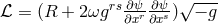
To obtain the Lagrangian for the metrical field,
within projective geometry was [383]
but then became generalized to
To obtain the Lagrangian for the metrical field, ![1 μν 2 L = 2[a(J)ψ,νψ,μg + b(J)ψ ] (107 )](article466x.gif)
![5 L = U (J )[R + W (J)ψ,νψ,μgμν + V (J)]. (108 )](article467x.gif)
 was replaced by
  ([384*], p. 57):
With
we arrive at:
where
([384*], p. 57):
With
we arrive at:
where ![5 L = U(J )[R + W (J)J,νJ,μgμν + V(J )]. (109 )](article470x.gif)

![[ 4 4 ] L = U (J ) R + 1J FrsF rs + J −1grs∇r ∂sJ + (W (J) − 1J −2)J,νJ,μgμν + V (J) , (111 ) 4 2](article472x.gif)
 are arbitrary functions. As can be seen from (110*), the 5-dimensional
curvature scalar used by Jordan and by Thiry (cf. the next Section 3.1.2) follows as the subcase
are arbitrary functions. As can be seen from (110*), the 5-dimensional
curvature scalar used by Jordan and by Thiry (cf. the next Section 3.1.2) follows as the subcase
 of the general expression (111*). Ludwig, at the time of writing the
preface to his book, e.g., in May 1951, seemingly did not know of Thiry’s paper of 1948 [604*]
nor of his PhD thesis published also in 1951: in his bibliography Thiry’s name and paper are
missing.
of the general expression (111*). Ludwig, at the time of writing the
preface to his book, e.g., in May 1951, seemingly did not know of Thiry’s paper of 1948 [604*]
nor of his PhD thesis published also in 1951: in his bibliography Thiry’s name and paper are
missing.
Pauli had browsed in Ludwig’s book and now distanced himself from his own papers on projective relativity of 1933 discussed briefly in Section 7.2.4 of Part I.44 He felt deceived:
“The deception consists in the belief that by the projective form, i.e., the homogeneous
coordinates, the shortcomings of Kaluza’s formulation have been repaired, and that one
has achieved something beyond Kaluza. At the time, in 1933, I did not know explicitly
the transition from Kaluza to the projective form (as in [20*]); it is too simple and banal
to the effect that the factual contents of both equivalent formulations could be somehow
different.” (letter of W. P. to P. Jordan, [490*], p. 735):45
3.1.2 Physical approach: Scalar-tensor theory
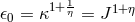
Toward the end of the second world war, Kaluza’s five- dimensional theory and projective relativity emerged
once again as vehicles for a new physical theory which, much later, came to be known as “scalar-tensor theory of
gravitation.”46
Cosmological considerations related to the origin of stars seem to have played the major role
for the building of a theory by P. Jordan in which the gravitational constant  is thought to be varying in (cosmological) time and thus replaced by a scalar function
[316]47.
The theory nicely fit with Dirac’s “large number hypothesis” [122, 123]. The fifteenth field variable in Kaluza’s
theory was identified by Jordan with this function, or in projective relativity, with the scalar:
is thought to be varying in (cosmological) time and thus replaced by a scalar function
[316]47.
The theory nicely fit with Dirac’s “large number hypothesis” [122, 123]. The fifteenth field variable in Kaluza’s
theory was identified by Jordan with this function, or in projective relativity, with the scalar:  by setting
  [321*]. In space-time, the field equations for the gravitational field
 , the electromagnetic 4-potential
  , and the
  -variable
  were derived by Jordan and
Müller48
to be:
were derived by Jordan and
Müller48
to be:
 . P. G. Bergmann, in a paper submitted
in August 1946 but published only in January of 1948, reported that work on a theory with a fifteenth field
variable had been going on in Princeton:
. P. G. Bergmann, in a paper submitted
in August 1946 but published only in January of 1948, reported that work on a theory with a fifteenth field
variable had been going on in Princeton:
“Professor Einstein and the present author had worked on that same idea several years earlier, but had finally rejected it and not published the abortive event” ([21*], p. 255).
It may be that at the time, they just did not have an idea for a physical interpretation like the one suggested by P. Jordan. Although there were reasons for studying the theory further, Bergmann pointed out that there is an “embarras de richesses” in the theory: too many constructive possibilities for a Lagrangian. Nonetheless, in his subsequent paper on “five-dimensional cosmology”, P. Jordan first stuck to the simplest Lagrangian, i.e. to the Ricci scalar in five dimensions [318*]. In this paper, Jordan also made a general comment on attempts within unitary field theory of the Einstein–Schrödinger-type to embed corpuscular matter into classical field theory (cf. chapter 6 with Section 6.1.1 below):
“The problem of the structure of matter can only be attacked as a problem in quantum
mechanics; nevertheless, investigations of the singularities of solutions of the field equations
retain considerable importance in this framework. […] the wave functions of matter must
be taken into account. Whether this program can be carried through, and to which
extent, in the sense of an extension of geometry (to which Schrödinger’s ideas related to
the meson field seem to provide an important beginning) is such a widespread question
[…]”.49
([318], p. 205).
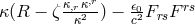
Jordan’s theory received wider attention after his and G. Ludwig’s books had been published in the early 1950s [319*, 384]. In a letter to Jordan mentioned, Pauli also questioned Jordan’s taking the five-dimensional curvature scalar as his Lagrangian. Actually, already in the first edition of his book, Jordan had accepted Pauli’s criticism and replaced (110*) by [compare with (109*)]:
He thus severed his “extended theory of gravitation” from Kaluza’s theory. He also displayed the Lagrangian ([319*], p. 139): but then set one of the two free parameters

 . One of those responding to this book was M. Fierz in
Basel [195*]. Before publication, he had corresponded with W. Pauli, sent him first versions of the paper and
eventually received Pauli’s placet; cf. the letter of Pauli to Fierz of 2 June 1956 in [492*], p. 578. In the
second edition of his book, Jordan also commented on a difficulty of his theory pointed out by
W. Pauli: instead of
. One of those responding to this book was M. Fierz in
Basel [195*]. Before publication, he had corresponded with W. Pauli, sent him first versions of the paper and
eventually received Pauli’s placet; cf. the letter of Pauli to Fierz of 2 June 1956 in [492*], p. 578. In the
second edition of his book, Jordan also commented on a difficulty of his theory pointed out by
W. Pauli: instead of  equally well
  with arbitrary function
  could serve as a
metric.50
This conformal invariance of the theory is preserved in the case that an electromagnetic field forms the
matter tensor. A problem for the interpretation of mathematical objects as physical variables results: by a
suitable choice of the conformal factor
could serve as a
metric.50
This conformal invariance of the theory is preserved in the case that an electromagnetic field forms the
matter tensor. A problem for the interpretation of mathematical objects as physical variables results: by a
suitable choice of the conformal factor  , a “constant” gravitational coupling function could be reached,
again. In his paper, M. Fierz suggested to either couple Jordan’s gravitational theory to point particles or
to a (quantum-) Klein–Gordon field in order to remove the difficulty. Fierz also claimed that Jordan had
overlooked a physical effect. According to him, a dielectricity “constant” of the vacuum could be introduced
, a “constant” gravitational coupling function could be reached,
again. In his paper, M. Fierz suggested to either couple Jordan’s gravitational theory to point particles or
to a (quantum-) Klein–Gordon field in order to remove the difficulty. Fierz also claimed that Jordan had
overlooked a physical effect. According to him, a dielectricity “constant” of the vacuum could be introduced
 from looking at Jordan’s field equations. His Lagrangian corresponded to
 with
with  . On the other hand, in the MKSA system of physical units,
the fine-structure constant is
. On the other hand, in the MKSA system of physical units,
the fine-structure constant is  . Thus, the fine-structure constant would depend on
 .
.
“Assumed that  be variable in cosmic spaces, then this variability must show up in the
redshift of light radiated from distant stars.” ([195], p. 134)51
be variable in cosmic spaces, then this variability must show up in the
redshift of light radiated from distant stars.” ([195], p. 134)51
Because this had not been observed, Fierz concluded that  . Both, Pauli and Fierz gave a low rating to Jordan’s
theory52
. Both, Pauli and Fierz gave a low rating to Jordan’s
theory52
Neither Pauli nor Fierz seem to have known that the mathematician Willy Scherrer at the university of Bern had suggested scalar-tensor theory already in 1941 before P. Jordan, and without alluding to Kaluza or Pauli’s projective formulation.53 Also, in 1949, Scherrer had suggested a more general Lagrangian [532]:

 is considered to be a scalar matter field. He had advised a student, K. Fink, to work on the Lagrangian
 [198]. The ensuing field equations correspond to those following
from Jordan’s Lagrangian if his parameter
[198]. The ensuing field equations correspond to those following
from Jordan’s Lagrangian if his parameter  ([319*] p. 140). Exact solutions in the static,
spherically symmetric case and for a homogeneous and isotropic cosmological model were published
in 1951 almost simultaneously by Fink (
([319*] p. 140). Exact solutions in the static,
spherically symmetric case and for a homogeneous and isotropic cosmological model were published
in 1951 almost simultaneously by Fink ( ) and Heckmann, Jordan & Fricke (
 )
[243].
)
[243].
In 1953, W. Scherrer asked Pauli to support another manuscript on unified field theory entitled “Grundlagen einer linearen Feldtheorie” for publication in Helvetica Physica Acta but apparently sent him only a reprint of a preliminary short note [534]. Pauli was loath to get involved and asked the editor of this journal, the very same M. Fierz, what the most appropriate answer to Scherrer could be. He also commented:
“Because according to my opinion all “unified field theories” are based on dubious ideas –
in particular it is a typically suspect idea of the great masters Einstein and Schrödinger
to add up the symmetric and antisymmetric parts of a tensor – I have to pose the question
[…].” (W. Pauli to M. Fierz, 15 Dec. 1953) ([491*], p. 390–391)54
Scherrer’s paper eventually was published in Zeitschrift für Physik [535]. In fact, he proposed a unified field theory based on linear forms, not on a quadratic form such as it is used in general relativity or Einstein–Schrödinger UFT. His notation for differential forms and tangent vectors living in two reference systems is non-standard. As his most important achievement he regarded “the absolutely invariant and at the same time locally exact conservation laws.” In his correspondence with Fierz, Pauli expressed his lack of understanding: “What he means with this, I do not know, because all generally relativistic field theories abound with energy laws”([491*], p. 403). H. T. Flint wrote a comment in which he claimed to have shown that Scherrer’s theory is kin to Einstein’s teleparallelism theory [213]. For studies of Kaluza’s theory in Paris (Jordan–Thiry theory) cf. Section 11.1.
3.2 Continued studies of Kaluza–Klein theory in Princeton, and elsewhere
As described in Section 6.3 of Part I, since 1927 Einstein and again in 1931 Einstein and Mayer55, within a calculus using 5-component tensorial objects in space-time, had studied Kaluza’s approach to a unification of gravitation and electromagnetism in a formal 5-dimensional space with Lorentz-signature. A decade later, Einstein returned to this topic in collaboration with his assistant Peter Bergmann [167*, 166]. The last two chapters of Bergmann’s book on relativity theory are devoted to Kaluza’s theory and its generalization ([20*]. Einstein wrote a foreword, in which he did not comment on “Kaluza’s unified field theory” as the theory is listed in the book’s index. He admitted that general relativity “[…] has contributed little to atomic physics and our understanding of quantum phenomena.” He hoped, however, that some of its features as were “general covariance of the laws of nature and their nonlinearity” could contribute to “overcome the difficulties encountered at present in the theory of atomic and nuclear processes” ([20*] p. V). Two years before Bergmann’s book appeared, Einstein already had made up his mind against the five-dimensional approach:
“The striving for most possible simplicity of the foundations of the theory has prompted
several attempts at joining the gravitational field and the electromagnetic field from a
unitary, formal point of view. Here, in particular, the five-dimensional theory of Kaluza
and Klein must be mentioned. Yet, after careful consideration of this possibility, I think it
more proper to accept the mentioned lack of inner unity, because it seems to me that the
embodiment of the hypotheses underlying the five-dimensional theory contains no less
arbitrariness than the original theory.”56
Nonetheless, in their new approach, Einstein and Bergmann claimed to ascribe “physical
reality to the fifth dimension whereas in Kaluza’s theory this fifth dimension was introduced
only in order to obtain new components of the metric tensor representing the electromagnetic
field” ([167], p. 683). Using ideas of O. Klein, this five-dimensional space was seen by them
essentially as a four-dimensional one with a small periodical strip or a tube in the additional
spacelike dimension affixed. The 4-dimensional metric then is periodic in the additional coordinate
 .57
With the fifth dimension being compact, this lessened the need for a physical interpretation of its empirical
meaning. Now, the authors partially removed Kaluza’s ‘cylinder condition’
.57
With the fifth dimension being compact, this lessened the need for a physical interpretation of its empirical
meaning. Now, the authors partially removed Kaluza’s ‘cylinder condition’  (cf. Section 4.2 of
Part I, Eq. (109)): they set
(cf. Section 4.2 of
Part I, Eq. (109)): they set  , but assumed
  and
and  : the electrodynamic
4-potential remains independent of
: the electrodynamic
4-potential remains independent of  . Due to the restriction of the covariance group (cf. Section 4.2,
Part I, Eq. (112)), in space-time many more possibilities for setting up a variational principle than
the curvature scalar of 5-dimensional space exist: besides the 4-dimensional curvature scalar
. Due to the restriction of the covariance group (cf. Section 4.2,
Part I, Eq. (112)), in space-time many more possibilities for setting up a variational principle than
the curvature scalar of 5-dimensional space exist: besides the 4-dimensional curvature scalar
 , Einstein & Bergmann list three further quadratic invariants:
 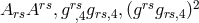 where
where  . The ensuing field equations for the fourteen variables
  and
and
 contain two new free parameters besides the gravitational and cosmological constants.
Scalar-tensor theory is excluded due to the restrictions introduced by the authors. Except for
the addition of some new technical concepts (p-tensors, p-differentiation) and the inclusion of
projective geometry, Bergmann’s treatment of Kaluza’s idea in his book did not advance the
field.
contain two new free parameters besides the gravitational and cosmological constants.
Scalar-tensor theory is excluded due to the restrictions introduced by the authors. Except for
the addition of some new technical concepts (p-tensors, p-differentiation) and the inclusion of
projective geometry, Bergmann’s treatment of Kaluza’s idea in his book did not advance the
field.
The mathematicians K. Yano and G. Vranceanu showed that Einstein’s and Bergmann’s generalization
may be treated as part of the non-holonomic UFT proposed by them [713, 681*]. Vranceanu considered
space-time to be a “non-holonomic” totally geodesic hypersurface in a 5-dimensional space  , i.e., the
hypersurface cannot be generated by the set of tangent spaces in each point. Besides the metric of
space-time
, i.e., the
hypersurface cannot be generated by the set of tangent spaces in each point. Besides the metric of
space-time  , a non-integrable differential form
  defining the hypersurface was introduced together with the additional assumption
  . The path of
a particle with charge
. The path of
a particle with charge  , mass
  and 5-vector
  was chosen to be a
geodesic tangent to the non-holonomic hypersurface. Thus
was chosen to be a
geodesic tangent to the non-holonomic hypersurface. Thus  , and Vranceanu then took
 . The electromagnetic field was defined as
  . Both Einstein’s
and Maxwell’s equations followed, separately, with the energy-momentum tensor of matter as
possible source of the gravitational field equations: “One can also assume that the energy tensor
. Both Einstein’s
and Maxwell’s equations followed, separately, with the energy-momentum tensor of matter as
possible source of the gravitational field equations: “One can also assume that the energy tensor
 be the sum of two tensors one of which is due to the electromagnetic field […]”. ([681*],
p. 525).58
be the sum of two tensors one of which is due to the electromagnetic field […]”. ([681*],
p. 525).58 His interpretation of the null geodesics which turn out to be independent of the electromagnetic field is in
the spirit of the time: “This amounts to suppose for light, or as well for the photon, that its charge be
null and its mass
His interpretation of the null geodesics which turn out to be independent of the electromagnetic field is in
the spirit of the time: “This amounts to suppose for light, or as well for the photon, that its charge be
null and its mass  be different from zero, a fact which is in accord with the hypothesis
of Louis de Broglie (Une nouvelle conception de la lumière; Hermann, Paris 1934).” ([681],
p. 524)59
More than a decade later, K. Yano and M. Ohgane generalized the non-holonomic UFT to arbitray
dimension:
be different from zero, a fact which is in accord with the hypothesis
of Louis de Broglie (Une nouvelle conception de la lumière; Hermann, Paris 1934).” ([681],
p. 524)59
More than a decade later, K. Yano and M. Ohgane generalized the non-holonomic UFT to arbitray
dimension:  -dimensional space is a non-holonomic hypersurface of
  -dimensional Riemannian
space. It is shown that the theory “[…] seems to contain all the geometries appearing in the
five-dimensional unified field theories proposed in the past and to suggest a natural generalization of
the six-dimensional unified field theories proposed by B. Hoffmann, J. Podolanski, and one
of the present authors” ([714], pp. 318, 325–326). They listed the theories by Kaluza–Klein,
Veblen–Hoffmann, Einstein–Mayer, Schouten–Dantzig, Vranceanu and Yano; cf. also Sections 3.1 and
11.2.1.
-dimensional Riemannian
space. It is shown that the theory “[…] seems to contain all the geometries appearing in the
five-dimensional unified field theories proposed in the past and to suggest a natural generalization of
the six-dimensional unified field theories proposed by B. Hoffmann, J. Podolanski, and one
of the present authors” ([714], pp. 318, 325–326). They listed the theories by Kaluza–Klein,
Veblen–Hoffmann, Einstein–Mayer, Schouten–Dantzig, Vranceanu and Yano; cf. also Sections 3.1 and
11.2.1.
B. Hoffmann derived the geodesic equations of a magnetic monopole in the framework of a 6-dimensional theory [277*]; cf. Section 11.2.1. The one who really made progress, although unintentionally and unnoticed at the time, was O. Klein who extended Abelian gauge theory for a particular non-Abelian group, which almost corresponds to SU(2) gauge theory [333]. For a detailed discussion of Klein’s contribution cf. [237].
Einstein unceasingly continued his work on the “total field” but was aware of inherent difficulties. In a letter to his friend H. Zangger in Zurich of 27 February 1938, he wrote:
“I still work as passionately even though most of my intellectual children, in a very young
age, end in the graveyard of disappointed hopes”. ([560*], p. 552)60
At first he was very much fascinated by the renewed approach to unified field theory by way of Kaluza’s idea. We learn this from the letter of 8 August 1938 to his friend Besso:
“After twenty years of vain searching, this year now I have found a promising field theory
which is a quite natural sequel to the relativistic gravitational theory. It is in line with
Kaluza’s idea about the essence of the electromagnetic field.” ([163*], p. 321)61
3.3 Non-local fields
3.3.1 Bi-vectors; generalized teleparallel geometry
In 1943, Einstein had come to the conclusion that the failure of “finding a unified theory of the physical
field by some generalization of the relativistic theory of gravitation” seemed to require “a decisive
modification of the fundamental concepts” ([165*], p. 1). He wanted to keep the four-dimensional space-time
continuum and the diffeomorphism group as the covariance group, but wished to replace the Riemannian
metric by a generalized concept. Together with the assistant at the Institute for Advanced Studies,
Valentine Bargmann , he set out to develop a new scheme involving
“bi-vector fields”. Unlike the concept of a bi-vector used by Schouten in 1924 ([537], p. 17) and ever
since in the literature, i.e., for the name of a special antisymmetric tensor, in the definition by
Einstein and Bargmann the concept meant a tensor depending on the coordinates of two points in
space-time, an object which would be called “bi-local” or “non-local”, nowadays. The two points,
alternatively, could be imagined to lie in the same manifold (“single space”), or in two different
spaces (“double space”). In the latter case, the coordinate transformations for each point are
independent.
In place of the Riemannian metric, a contravariant bi-vector  is defined via


 for a simple “bi-vector”
  is given by:
Already here a problem was mentioned in the paper: there exist too many covariant geometric objects
available for deriving field equations. This is due to the possibility to form covariant quantities containing
only first order derivatives like the tensorial quantity:
is given by:
Already here a problem was mentioned in the paper: there exist too many covariant geometric objects
available for deriving field equations. This is due to the possibility to form covariant quantities containing
only first order derivatives like the tensorial quantity: 
 . In order to cut
down on this wealth, a new operation called “rimming” was introduced which correlated a new
“bi-vector”
. In order to cut
down on this wealth, a new operation called “rimming” was introduced which correlated a new
“bi-vector”  with
with  by multiplying it from left and right by tensors of full rank
  where each is taken from one of the two manifolds (now Greek indices refer to the two different
points)62:
All tensors
where each is taken from one of the two manifolds (now Greek indices refer to the two different
points)62:
All tensors 
 obtained by rimming
  were considered as different representations of the same field. The
rimming of a contravariant “bi-vector” was done similarly by multiplying from the left with
were considered as different representations of the same field. The
rimming of a contravariant “bi-vector” was done similarly by multiplying from the left with  and from
the right with tensors
and from
the right with tensors  . In order that (118*), (119*) remain invariant under rimming, the relations
 , must hold. A comparison of (120*) and (121*) shows that a coordinate
transformation can be combined with a rimming operation “in such a way that the bi-vector
components remain invariant – i.e., behave like scalars under the resultant transformation” ([165*],
p. 4).
, must hold. A comparison of (120*) and (121*) shows that a coordinate
transformation can be combined with a rimming operation “in such a way that the bi-vector
components remain invariant – i.e., behave like scalars under the resultant transformation” ([165*],
p. 4).
As a possible field equation, the authors now introduced “tensorial four-point equations”:
If
 is treated as a matrix, it is easy to see that all higher-order tensorial equations (6, 8, …-point) are
dependent on the four-point equation. Next, the authors showed that by a special rimming operation
is treated as a matrix, it is easy to see that all higher-order tensorial equations (6, 8, …-point) are
dependent on the four-point equation. Next, the authors showed that by a special rimming operation  can be transformed into
  such that the corresponding space-time is flat. The trace on (i,j) in (122*)
leads to a scalar equation:
This equations apparently allows for non-flat solutions (cf. Eq. (13), p. 6 in [165]).
such that the corresponding space-time is flat. The trace on (i,j) in (122*)
leads to a scalar equation:
This equations apparently allows for non-flat solutions (cf. Eq. (13), p. 6 in [165]).

In another paragraph, the authors returned to the “single space”-version. Here, a symmetry condition is
demanded:  . Now, the tensorial p-point equations admit the special case that the two points
(coordinates
. Now, the tensorial p-point equations admit the special case that the two points
(coordinates  ) coincide. By a suitable rimming operation
  was reached where
  is the
matrix diag
is the
matrix diag  . The rimming operations were performed with representations of the Lorentz
group. Also, mixed bi-vectors
. The rimming operations were performed with representations of the Lorentz
group. Also, mixed bi-vectors  were introduced and a tensorial three-point equation had to be
satisfied:
were introduced and a tensorial three-point equation had to be
satisfied:

In a continuation of this paper, Einstein explicitly introduced the concept of connection: “I show that
just as in the case of the infinitesimal theory this theory can be made very simple by separating the
concepts and relations into those based exclusively on the affine connection and those where the affine
connection is specialized by hypotheses on the structure of the field” ([146*], p. 15). The mixed
bi-vector  is interpreted as the (non-infinitesimal) affine connection because the relation

 and
and
 .63
Two conditions are to be fulfilled: the displacement of a vector from
.63
Two conditions are to be fulfilled: the displacement of a vector from  to
to  and back does not change
it, and “the scalar product of a covariant and a contravariant vector is invariant with respect to the affine
connection”. This led to
Taking into account the rimming operation, it is seen that (125*) and (126*) are invariant with respect to
rimming. Again a tensorial three-point equation was written down which, in matrix form, reads as:
The consequences of (127*) were the same as for the 4-point equation before: space-time is flat. To escape
this conclusion, the trace of (127*) could also be used “as a possible choice of a field law of a bi-vector field”
([146*], p. 17). Furthermore, the symmetry of the metric could be replaced by the more general:
In the remaining part of the paper, various possible cases were discussed and a new concept introduced:
“volume invariance”. For this, the rimming matrices were restricted to have determinant
and back does not change
it, and “the scalar product of a covariant and a contravariant vector is invariant with respect to the affine
connection”. This led to
Taking into account the rimming operation, it is seen that (125*) and (126*) are invariant with respect to
rimming. Again a tensorial three-point equation was written down which, in matrix form, reads as:
The consequences of (127*) were the same as for the 4-point equation before: space-time is flat. To escape
this conclusion, the trace of (127*) could also be used “as a possible choice of a field law of a bi-vector field”
([146*], p. 17). Furthermore, the symmetry of the metric could be replaced by the more general:
In the remaining part of the paper, various possible cases were discussed and a new concept introduced:
“volume invariance”. For this, the rimming matrices were restricted to have determinant 


 . Another
field law then was proposed:
In a note in proof Einstein remarked that “W. Pauli and V. Bargmann have meanwhile succeeded in
proving that (129*), too, admits only “flat space” solutions”([146], p. 23). He slightly changed the equation
into:
and ended the paper (and his publications on “bi-vectors”) by stating: “At present, the author, in
collaboration with W. Pauli, is trying to find out whether this equation has non-trivial solutions”. Thus,
besides a new mathematical scheme, and Einstein’s method of “trial and error” for finding field equations,
no progress in terms of unified field theory had been achieved.
. Another
field law then was proposed:
In a note in proof Einstein remarked that “W. Pauli and V. Bargmann have meanwhile succeeded in
proving that (129*), too, admits only “flat space” solutions”([146], p. 23). He slightly changed the equation
into:
and ended the paper (and his publications on “bi-vectors”) by stating: “At present, the author, in
collaboration with W. Pauli, is trying to find out whether this equation has non-trivial solutions”. Thus,
besides a new mathematical scheme, and Einstein’s method of “trial and error” for finding field equations,
no progress in terms of unified field theory had been achieved.


The only physicist outside of Princeton who expressed an interest in this discovery of “a new form of geometrical connection of a continuum, the distant affine connection” was Schrödinger in Dublin. In his paper, he set out to
“[…] show how the new geometrical structure emerges, by generalization, from the one that was at the basis of Einstein’s ‘Distant Parallelism’ (Fernparallelismus), and consisted in the natural union of an integrable (but in general non-symmetric) infinitesimal affine connection and a (in general not flat) Riemannian metric” ([550], p. 143).
He rewrote Einstein’s mixed bi-vector with the help of the tetrads used in teleparallel geometry:
Note that Schrödinger denoted the tetrad by
 with Latin indices
  for the number of the leg,
and Greek space-time indices such that
for the number of the leg,
and Greek space-time indices such that  . By comparing the parallel displacement of a
4-vector
. By comparing the parallel displacement of a
4-vector  with
with  he arrived at his interpretation of
  as a connection.
As the relation between the affine connection – which he called “infinitesimal connection” – and the
bi-vector connection, named “distant connection”, he took:
In the following paper with Friedrich Mautner, scholar at the Dublin Institute for Advanced Studies, who
already had been acknowledged as coworker in the first publication, Schrödinger likened Einstein’s
three-point tensor in (127*) to the curvature tensor: the three-point matrices of a distant affinity perform a
transfer from the point
as a connection.
As the relation between the affine connection – which he called “infinitesimal connection” – and the
bi-vector connection, named “distant connection”, he took:
In the following paper with Friedrich Mautner, scholar at the Dublin Institute for Advanced Studies, who
already had been acknowledged as coworker in the first publication, Schrödinger likened Einstein’s
three-point tensor in (127*) to the curvature tensor: the three-point matrices of a distant affinity perform a
transfer from the point 
 via
via  back to the starting point
  . This is analogous to parallel
transfer around a triangle formed by the points
. This is analogous to parallel
transfer around a triangle formed by the points  ; the change of a vector thus transported along the
closed circuit is proportional to the curvature tensor, if it is skew symmetric also in the first pair of
indices ([399], pp. 224–225). This analogy was carried on further; a formula corresponding
to (59*) of Section 2.3.1 was derived, with the symmetric affine connection replaced by the
Christoffel symbols and torsion by contorsion, i.e., by
; the change of a vector thus transported along the
closed circuit is proportional to the curvature tensor, if it is skew symmetric also in the first pair of
indices ([399], pp. 224–225). This analogy was carried on further; a formula corresponding
to (59*) of Section 2.3.1 was derived, with the symmetric affine connection replaced by the
Christoffel symbols and torsion by contorsion, i.e., by  . Both cases in (128*)
were treated and tentative field equations including a cosmological constant written down. The
paper ended with the sentence: “Are these equations likely to give an appropriate description of
physical fields?” As is known now, the answer to this question should have been “no”. Thus, in
this context, Schrödinger’s papers also did not bring progress for UFT; nevertheless, they
helped to make Einstein’s papers more readable. The subject was also taken up by a Romanian
mathematician, M. Haimovici (1906 – 1973), who instead introduced a space of point-couples,
introduced axioms for defining a connection there, and established a relation to work by E. Cartan
[239].
. Both cases in (128*)
were treated and tentative field equations including a cosmological constant written down. The
paper ended with the sentence: “Are these equations likely to give an appropriate description of
physical fields?” As is known now, the answer to this question should have been “no”. Thus, in
this context, Schrödinger’s papers also did not bring progress for UFT; nevertheless, they
helped to make Einstein’s papers more readable. The subject was also taken up by a Romanian
mathematician, M. Haimovici (1906 – 1973), who instead introduced a space of point-couples,
introduced axioms for defining a connection there, and established a relation to work by E. Cartan
[239].
3.3.2 From Born’s principle of reciprocity to Yukawa’s non-local field theory
Much earlier, Max Born had followed a different if not entirely unrelated conceptual course: in 1938, he had
introduced a “principle of reciprocity”: “ […] each general law on the  -space has an ’inverse image’ in the
 -space, in the first instance the laws of relativity” ([38], p. 327). In this note in Nature, Born added a
Lorentzian metric
-space, in the first instance the laws of relativity” ([38], p. 327). In this note in Nature, Born added a
Lorentzian metric  in momentum space satisfying as well the corresponding Einstein field
equations (cf. Section 4.2). Infeld in Princeton wanted to get some further information about this principle
of reciprocity from Born, who was afraid that his idea be seized by the “terribly clever people over there”.
However, in his letter to Einstein of 11 April 1938, he described his joint work with Klaus Fuchs: to
derive a “super-mechanics” with an 8-dimensional metric in phase space. A new fundamental
(“natural”) constant appeared leading to both an absolute length and an absolute momentum ([168*],
pp. 182–184). In a way, Born’s formalism came near to Einstein’s “double space” in his bi-vector
theory.
in momentum space satisfying as well the corresponding Einstein field
equations (cf. Section 4.2). Infeld in Princeton wanted to get some further information about this principle
of reciprocity from Born, who was afraid that his idea be seized by the “terribly clever people over there”.
However, in his letter to Einstein of 11 April 1938, he described his joint work with Klaus Fuchs: to
derive a “super-mechanics” with an 8-dimensional metric in phase space. A new fundamental
(“natural”) constant appeared leading to both an absolute length and an absolute momentum ([168*],
pp. 182–184). In a way, Born’s formalism came near to Einstein’s “double space” in his bi-vector
theory.
About a decade later, in 1947, H. Yukawa in an attempt to arrive at a theory of elementary particles,
used exactly this “double space”-approach: “[…] the field in our case is not necessarily a function of  alone, but may depend on
  also. […] The generalized field can include not only the electromagnetic field
and various types of meson fields but also the so-called pair-fields such as the meson pair field and the
electron-neutrino field” ([716], p. 211–212). It seems that he saw his non-local field theory as introducing
new degrees of freedom and leading a step away from the point-particle concept: a possibility for avoiding
infinite self-energies. During his stay at the Princeton Institute for Advanced Study (PIAS) in 1948/49,
Yukawa must have learned about Born’s reciprocity principle and work around it [45, 46, 47],
refered to it (cf. [718]) and embarked on his quantum-theory of non-local fields. In general, his
theory now corresponded to the “single space” of Einstein and Bargmann: operators
also. […] The generalized field can include not only the electromagnetic field
and various types of meson fields but also the so-called pair-fields such as the meson pair field and the
electron-neutrino field” ([716], p. 211–212). It seems that he saw his non-local field theory as introducing
new degrees of freedom and leading a step away from the point-particle concept: a possibility for avoiding
infinite self-energies. During his stay at the Princeton Institute for Advanced Study (PIAS) in 1948/49,
Yukawa must have learned about Born’s reciprocity principle and work around it [45, 46, 47],
refered to it (cf. [718]) and embarked on his quantum-theory of non-local fields. In general, his
theory now corresponded to the “single space” of Einstein and Bargmann: operators  )
depended on “two sets of real variables” (in the same space) [719, 720, 721]. According to
Yukawa: “
)
depended on “two sets of real variables” (in the same space) [719, 720, 721]. According to
Yukawa: “ coincide with the ordinary coordinates
  in the limit of local field, so that the
dependence on
in the limit of local field, so that the
dependence on  describes the asymptotic behavior and the dependence on
  characterizes the
internal structure or inertial motion” ([722], p. 3 ). At this time, both Yukawa and Einstein lived
in Princeton and got to know each other. It can reasonably be doubted, though, that they
took note of each other’s scientific work except superficially. In 1947, Yukawa possibly had not
the least inkling of the Einstein–Bargmann paper of 1944. Of course, Bargmann in Princeton
then could have told him. In the special issue of Review of Modern Physics for Einstein’s 70th
birthday in 1949, Max Born in Edinburgh dedicated an article about his reciprocity principle to
Einstein:
characterizes the
internal structure or inertial motion” ([722], p. 3 ). At this time, both Yukawa and Einstein lived
in Princeton and got to know each other. It can reasonably be doubted, though, that they
took note of each other’s scientific work except superficially. In 1947, Yukawa possibly had not
the least inkling of the Einstein–Bargmann paper of 1944. Of course, Bargmann in Princeton
then could have told him. In the special issue of Review of Modern Physics for Einstein’s 70th
birthday in 1949, Max Born in Edinburgh dedicated an article about his reciprocity principle to
Einstein:
“The theory of elementary particles which I propose in the following pages is based on the current conceptions of quantum mechanics and differs widely from the ideas which Einstein himself has developed in regard to this problem. […] It can be interpreted as a rational generalization of his (“special”) theory of relativity.” ([40], p. 463)
Right next to Born’s article, one by Yukawa was placed which dealt with meson theory. He made only a cryptic remark about his non-local field theory when expressing the then prevailing ignorance about elementary particle theory:
“Probably we need a broader background (such as the five-dimensional space or the quantized phase space) for field theory in order to cope with these problems, although it is premature to say anything definite in this connection.” ([717], p.479)
He then gave references to his papers on non-local field theory. In a letter of 23 January 1949, Born informed Einstein also privately about his theory of elementary particles:
The laws of nature are invariant not only with regard to the relativistic transformations
but also with regard to the substitutions  […]. All amounts to replace
your fundamental invariant
[…]. All amounts to replace
your fundamental invariant  by the symmetrical quantity
  where
where
 .
.  is an operator, the integer eigenvalues of which are the distances […].”
([168*], p. 242.)64
is an operator, the integer eigenvalues of which are the distances […].”
([168*], p. 242.)64
This story shows that a very loose kinship existed between the Einstein–Bargmann “bi-vector” method and Yukawa’s non-local field theory with Born’s reciprocity theory in the middle. Although some of those involved were in direct personal contact, no concrete evidence for a conscious transfer of ideas could be established.
 |
 |
 |
Living Rev. Relativity, 17 (2014), 5, doi:10.12942/lrr-2014-5, URL (accessed <date>): http://www.livingreviews.org/lrr-2014-5.
 This work is licensed under a Creative Commons License.
© The author(s), except where otherwise noted.
This work is licensed under a Creative Commons License.
© The author(s), except where otherwise noted.