Relativistic shock heating in planar, cylindrical and spherical geometry

6.1 Relativistic shock heating in planar, cylindrical and spherical geometry

Shock heating of a cold fluid in planar, cylindrical, or spherical geometry has been used since the early developments of numerical relativistic hydrodynamics as a test case for hydrodynamic codes, because it has an analytical solution ([26 ] in planar symmetry, [183

] in cylindrical and spherical symmetry), and because it involves the propagation of a strong relativistic shock wave.

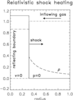
In planar geometry, an initially homogeneous, cold (i.e., $𝜀 ≈ 0$ ) gas with coordinate velocity v₁ and Lorentz factor W₁ is supposed to hit a wall, while in the case of cylindrical and spherical geometry the gas flow converges towards the axis or the center of symmetry. In all three cases the reflection causes compression and heating of the gas as kinetic energy is converted into internal energy. This occurs in a shock wave, which propagates upstream. Behind the shock the gas is at rest (v₂ = 0). Due to conservation of energy across the shock, the gas has a specific internal energy given by

The compression ratio $σ$ of shocked and unshocked gas follows from

where $γ$ is the adiabatic index of the equation of state. The shock velocity is given by

In the unshocked region ( $r ∈ [V t,∞ [ s$ ) the pressure-less gas flow is self-similar and has a density distribution given by

where $α$ = 0, 1, 2 for planar, cylindrical, or spherical geometry, and where $ρ0$ is the density of the inflowing gas at infinity (see Figure 5

Figure 5: Schematic solution of the shock heating problem in spherical geometry. The initial state consists of a spherically symmetric flow of cold (p = 0) gas of unit rest mass density having a highly relativistic inflow velocity everywhere. A shock is generated at the center of the sphere, which propagates upstream with constant speed. The post-shock state is constant and at rest. The pre-shock state, where the flow is self-similar, has a density which varies as $ρ$ = (1 + t/r)² with time t and radius r.

In the Newtonian case the compression ratio $σ$ of shocked and unshocked gas cannot exceed a value of $σmax = (γ + 1)∕(γ − 1)$ independently of the inflow velocity. This is different for relativistic flows, where $σ$ grows linearly with the flow Lorentz factor and becomes infinite as the inflowing gas velocity approaches to speed of light.

The maximum flow Lorentz factor achievable for a hydrodynamic code with acceptable errors in the compression ratio $σ$ is a measure of the code’s quality. Table 6 contains a summary of the results obtained for the shock heating test by various authors.

Explicit finite difference techniques based on a non-conservative formulation of the hydrodynamic equations and on non-consistent artificial viscosity [50 , 123 , 10 ] (or even consistent artificial viscosity [10 ]) are able to handle flow Lorentz factors up to $≈$ 10 with moderately large errors ( $σerror ≈ 1– 3%$ ) at best [297 , 187 ]. Norman and Winkler [214 ] got very good results ( $σerror ≈ 0.01%$ ) for a flow Lorentz factor of 10 using consistent artificial viscosity terms and an implicit adaptive mesh method.

The performance of explicit codes improved significantly when numerical methods based on Riemann solvers were introduced [179 , 176 , 83 , 257 , 84 , 181 , 89 ]. More recently, HRSC methods based on symmetric discretizations [71 , 10 ] have also demonstrated the same capability to describe highly relativistic flows. For some of these codes the maximum flow Lorentz factor is only limited by the precision by which numbers are represented on the computer used for the simulation [74 , 295 , 6 , 10 ].

Schneider et al. [257 ] have compared the accuracy of a code based on the RHLLE Riemann solver with different versions of relativistic FCT codes for inflow Lorentz factors in the range 1.5 to 50. They find that the error in $σ$ is reduced by a factor of two when using HLL. Further tests of the (1D) RHLLE method were performed by Rischke et al. [245 , 247 , 246 ] who considered expansion into vacuum, semi-infinite colliding slabs, and spherically and cylindrically symmetric expansions for equations of state for both thermodynamically normal and anomalous matter (see Section 7.3). In the latter two test cases RHLLE transport is done in the radial direction while corrections due to geometry are implemented via Sod’s method. Rischke et al. [245 , 247 ] also present a detailed comparison of the RHLLE method and relativistic extensions [113 ] of flux-corrected transport (FCT) algorithms [33 , 35 , 34 ]. They find that not all versions of the numerical algorithms explored in their investigation can be straightforwardly applied. Moreover, numerical parameters like the grid spacing or the antidiffusion coefficients (for FCT SHASTA) must be chosen with care, in order to produce solutions which are free of numerical artifacts. Studying the “slab-on-slab” collision test problem (up to flow Lorentz factors of 2.3) they particularly find [247 ] that analytical solutions are reproduced remarkably well with RHLLE and also with FCT SHASTA, provided the numerical diffusion is sufficiently large (i.e., when the antidiffusion in SHASTA is chosen sufficiently small).

Within SPH methods, Chow and Monaghan [53 ] have obtained results comparable to those of HRSC methods ( $σerror < 2 × 10−3$ ) for flow Lorentz factors up to 70, using a relativistic SPH code with Riemann solver guided dissipation. Sieglert and Riffert [262 ] have succeeded in reproducing the post-shock state accurately for inflow Lorentz factors of 1000 with a code based on a consistent formulation of artificial viscosity. However, the dissipation introduced by SPH methods at the shock transition is very large (10–12 particles in the code of [262 ]; 20–24 in the code of [53 ]) compared with the typical dissipation of HRSC methods (see below).

Table 6: Summary of relativistic shock heating test calculations by various authors in planar ( $α$ = 0), cylindrical ( $α$ = 1), and spherical ( $α$ = 2) geometry. W_max and $σ error$ are the maximum inflow Lorentz factor and compression ratio error extracted from tables and figures of the corresponding reference. W_max should only be considered as indicative of the maximum Lorentz factor achievable by the respective method. Methods are described in Sections 3 and 4, and their basic properties are summarized in Section 5 (Tables 3, 4, and 5).

References	$α$	Method	W_max	$σerror$ [%]
Centrella and Wilson (1984) [50 ]	0	AV-mono	2.29	$≈$ 10

Hawley et al. (1984) [123 ]	0	AV-mono	4.12	$≈$ 10

Norman and Winkler (1986) [214 ]	0	cAV-implicit	10.0	0.01

McAbee et al. (1989) [187 ]	0	AV-mono	10.0	2.6

Martí et al. (1991) [179 ]	0	Roe type-l	23	0.2

Marquina et al. (1992) [176 ]	0	LCA-phm	70	0.1

Eulderink (1993) [83 ]	0	Roe–Eulderink	625	$≤$ 0.1¹

Schneider et al. (1993) [257 ]	0	RHLLE	10⁶	0.2²

	0	SHASTA-c	10⁶	0.5³

Dolezal and Wong (1995) [74 ]	0	LCA-eno	7.0 × 10⁵	$≤$ 0.1⁴

Martí and Müller (1996) [181 ]	0	rPPM	224	0.03

Falle and Komissarov (1996) [89 ]	0	Falle–Komissarov	224	$≤$ 0.1⁵

Romero et al. (1996) [250 ]	2	Roe type-l	2236	2.2

Martí et al. (1997) [183 ]	1	MFF-ppm	70	1.0

Chow and Monaghan (1997) [53 ]	0	SPH-RS-c	70	0.2

Wen et al. (1997) [295 ]	2	rGlimm	224	10^–9

Donat et al. (1998) [75 ]	0	MFF-eno	224	$≤$ 0.1⁶

Aloy et al. (1999) [6 ]	0	MFF-ppm	2.4 × 10⁵	3.5⁷

Sieglert and Riffert (1999) [262 ]	0	SPH-cAV-c	1000	$≤$ 0.1⁸

Del Zanna and Bucciantini (2002) [71 ]	0	sCENO	224	2.3⁹

Anninos and Fragile (2002) [10 ]	0	cAV-mono	4.12	13.3

	0	NOCD	2.4 × 10⁵	0.1

Get Flash to see this player.

Figure 6: mpg-Movie (711 KB) The evolution of the density distribution for the shock heating problem with an inflow velocity v₁ = –0.99999 c in Cartesian coordinates. The reflecting wall is located at x = 0. The adiabatic index of the gas is 4/3. For numerical reasons, the specific internal energy of the inflowing cold gas is set to a small finite value ( $𝜀1$ = 10^–7 W₁). The final frame of the movie also shows the analytical solution (blue lines). The simulation has been performed on an equidistant grid of 100 zones.

The performance of a HRSC method based on a relativistic Riemann solver is illustrated by means of a movie (Figure 6 ) for the planar shock heating problem for an inflow velocity v₁ = –0.99999 c (W₁ $≈$ 223). These results are obtained with the relativistic code rPPM used in [181 ] and provided in Section 9.4.3.

The shock wave is resolved by three zones and there are no post-shock numerical oscillations. The density increases by a factor $≈$ 900 across the shock. Near x = 0 the density distribution slightly undershoots the analytical solution (by $≈$ 8%) due to the numerical effect of wall heating. The profiles obtained for other inflow velocities are qualitatively similar. The mean relative error of the compression ratio $σ error$ is smaller than 10^–3, and, in agreement with other codes based on a Riemann solver, the accuracy of the results does not exhibit any significant dependence on the Lorentz factor of the inflowing gas. The quality of the results obtained with high-order symmetric schemes [10 , 71 ] is similar.

Some authors have considered the problem of shock heating in cylindrical or spherical geometry using adapted coordinates to test the numerical treatment of geometrical factors [250 , 183 , 295 ]. Aloy et al. [6 ] have considered the spherically symmetric shock heating problem in 3D Cartesian coordinates as a test case for both the directional splitting and the symmetry properties of their code GENESIS. The code is able to handle this test up to inflow Lorentz factors of the order of 700.

In the shock reflection test, conventional schemes often give numerical approximations which exhibit a consistent O(1) error for the density and internal energy in a few cells near the reflecting wall. This ‘overheating’, as it is known in classical hydrodynamics [213 ], is a numerical artifact which is considerably reduced when Marquina’s scheme is used [76 ]. In passing we note that the strong overheating found by Noh [213 ] for the spherical shock reflection test using PPM (Figure 24 in [213 ]) is not a problem of PPM, but of his implementation of PPM. When properly implemented, PPM gives a density undershoot near the origin of about 9% in case of a non-relativistic flow. The piece-wise linear method described in [250 ] gives an undershoot of 14% in case of ultra-relativistic flows (e.g., Table 1 and Figure 1 in [250 ]).