Problem 1 was a demanding problem for relativistic hydrodynamic codes in the mid-eighties [50![]() , 123
, 123![]() ],
while Problem 2 is a challenge even for today’s state-of-the-art codes. The analytical solution of both
problems can be obtained with program RIEMANN (see Section 9.4).
],
while Problem 2 is a challenge even for today’s state-of-the-art codes. The analytical solution of both
problems can be obtained with program RIEMANN (see Section 9.4).
| Problem 1 | Problem 2 | |||||
| Left | Right | Left | Right | |||
| |
13.33 | 0.00 | 1000.00 | 0.01 | ||
| |
10.00 | 1.00 | 1.00 | 1.00 | ||
| |
0.00 | 0.00 | 0.00 | 0.00 | ||
| 0.72 | 0.960 | |||||
| 0.11 t | 0.026 t | |||||
| 0.83 | 0.986 | |||||
| 5.07 | 10.75 | |||||
In Problem 1, the decay of the initial discontinuity gives rise to a dense shell of matter with
velocity ![]() = 0.72 (
= 0.72 (![]() = 1.38) propagating to the right. The shell trailing a shock
wave of speed
= 1.38) propagating to the right. The shell trailing a shock
wave of speed ![]() = 0.83 increases its width
= 0.83 increases its width ![]() according to
according to ![]() = 0.11 t, i.e.,
at time t = 0.4 the shell covers about 4% of the grid (
= 0.11 t, i.e.,
at time t = 0.4 the shell covers about 4% of the grid (![]() ). Tables 8 and 9 give a
summary of the references where this test was considered for non-HRSC and HRSC methods,
respectively.
). Tables 8 and 9 give a
summary of the references where this test was considered for non-HRSC and HRSC methods,
respectively.
| References | Dim. | Method | Comments |
| Centrella and Wilson (1984) [50 |
1D | AV-mono | Stable profiles without oscillations; |
| velocity overestimated by 7%. | |||
| Hawley et al. (1984) [123 |
1D | AV-mono | Stable profiles without oscillations; |
| Dubal (1991)10 [77 |
1D | FCT-lw | 10–12 zones at the CD; |
| velocity overestimated by 4.5%. | |||
| Mann (1991) [172 |
1D | SPH-AV-0,1,2 | Systematic errors in the rarefaction |
| wave and the constant states; | |||
| large amplitude spikes at the CD; | |||
| excessive smearing at the shell. | |||
| Laguna et al. (1993) [150 |
1D | SPH-AV-0 | Large amplitude spikes at the CD; |
| van Putten (1993)11 [287 |
1D | van Putten | Stable profiles; |
| excessive smearing, especially of the | |||
| CD ( |
|||
| Schneider et al. (1993) [257 |
1D | SHASTA-c | Non-monotonic intermediate states; |
| 200 zones. | |||
| Chow and Monaghan (1997) [53 |
1D | SPH-RS-c | Monotonic profiles; |
| excessive smearing of CD and shock. | |||
| Siegler and Riffert (1999) [262 |
1D | SPH-cAV-c | Correct constant states; |
| large amplitude spikes at the CD; | |||
| excessive smearing of shock. | |||
| Muir (2002) [204 |
1D, 3D | SPH-RS-gr | Monotonic profiles; |
| excessive smearing of CD and shock. | |||
| Anninos and Fragile (2002) [10 |
1D, 3D | cAV-mono | Stable profiles without oscillations; |
| correct constant states. | |||
| References | Dim. | Method | Comments12 |
| Eulderink (1993) [83 |
1D | Roe–Eulderink | Correct |
| 4 zones in CD. | |||
| Schneider et al. (1993) [257 |
1D | RHLLE | |
| with 200 zones. | |||
| Martí and Müller (1996) [181 |
1D | rPPM | Correct |
| 6 zones in CD. | |||
| Martí et al. (1997) [183 |
1D, 2D | MFF-ppm | Correct |
| 6 zones in CD. | |||
| Wen et al. (1997) [295 |
1D | rGlimm | No diffussion at discontinuities. |
| Yang et al. (1997) [303 |
1D | rBS | Stable profiles. |
| Donat et al. (1998) [75 |
1D | MFF-eno | Correct |
| 8 zones in CD. | |||
| Aloy et al. (1999) [6 |
3D | MFF-ppm | Correct |
| 2 zones in CD. | |||
| Font et al. (1999) [93 |
1D, 3D | MFF-l | Correct |
| 12–14 zones in CD. | |||
| 1D, 3D | Roe type-l | Correct |
|
| 12–14 zones in CD. | |||
| 1D, 3D | Flux split | ||
| 8 zones in CD. | |||
| Del Zanna and Bucciantini (2002) | 1D | sCENO | Correct |
| 6 zones in CD. | |||
| Anninos and Fragile (2002) | 1D, 3D | NOCD | Correct |
| 14 zones in CD. | |||
Using artificial viscosity techniques, Centrella and Wilson [50] were able to reproduce the analytical
solution with a 7% overshoot in ![]() , whereas Hawley et al. [123
, whereas Hawley et al. [123![]() ] found a 16% error in the shell density.
However, when implementing a consistent formulation of artificial viscosity, like in the method
developed by Anninos and Fragile [10
] found a 16% error in the shell density.
However, when implementing a consistent formulation of artificial viscosity, like in the method
developed by Anninos and Fragile [10![]() ], it is possible to capture the constant states in a stable
manner and without noticeable errors (e.g., the shell density is underestimated by less than
2%).
], it is possible to capture the constant states in a stable
manner and without noticeable errors (e.g., the shell density is underestimated by less than
2%).
The results obtained with early relativistic SPH codes [172![]() ] were affected by systematic errors in the
rarefaction wave and the constant states, large amplitude spikes at the contact discontinuity, and large
smearing. Smaller systematic errors and spikes are obtained with Laguna et al.’s (1993) code [150
] were affected by systematic errors in the
rarefaction wave and the constant states, large amplitude spikes at the contact discontinuity, and large
smearing. Smaller systematic errors and spikes are obtained with Laguna et al.’s (1993) code [150![]() ]. This
code also leads to a large density overshoot in the shell. Much cleaner states are obtained with the methods
of Chow and Monaghan (1997) [53
]. This
code also leads to a large density overshoot in the shell. Much cleaner states are obtained with the methods
of Chow and Monaghan (1997) [53![]() ] and Siegler and Riffert (1999) [262
] and Siegler and Riffert (1999) [262![]() ], both based on conservative
formulations of the SPH equations. For Chow and Monaghan’s (1997) method [53
], both based on conservative
formulations of the SPH equations. For Chow and Monaghan’s (1997) method [53![]() ] the spikes at
the contact discontinuity disappear but at the cost of an excessive smearing. This smearing
can also be observed in Muir [204
] the spikes at
the contact discontinuity disappear but at the cost of an excessive smearing. This smearing
can also be observed in Muir [204![]() ] (see Figures 8
] (see Figures 8![]() and 9
and 9![]() ), who used the general relativistic,
conservative SPH formulation of Monaghan and Price [202], and the dissipation method of Chow and
Monaghan [53
), who used the general relativistic,
conservative SPH formulation of Monaghan and Price [202], and the dissipation method of Chow and
Monaghan [53![]() ] to simulate Problem 1 assuming a Minkowski spacetime. Generally speaking,
shock profiles obtained with relativistic SPH codes are smeared out more than those computed
with HRSC methods, the shocks modelled by SPH typically being covered by more than 10
zones.
] to simulate Problem 1 assuming a Minkowski spacetime. Generally speaking,
shock profiles obtained with relativistic SPH codes are smeared out more than those computed
with HRSC methods, the shocks modelled by SPH typically being covered by more than 10
zones.
Van Putten has considered a similar initial value problem with somewhat more extreme conditions
(![]() ,
, ![]() ) and with a transversal magnetic field. For suitable choices of the smoothing
parameters his results are accurate and stable, although discontinuities appear to be more smeared than
with typical HRSC methods (6–7 zones for the strong shock wave;
) and with a transversal magnetic field. For suitable choices of the smoothing
parameters his results are accurate and stable, although discontinuities appear to be more smeared than
with typical HRSC methods (6–7 zones for the strong shock wave; ![]() 50 zones for the contact
discontinuity).
50 zones for the contact
discontinuity).
A movie (Figure 10![]() ) shows the Problem 1 blast wave evolution obtained with a modern HRSC method
(the relativistic PPM method introduced in Section 3.1; code rPPM provided in Section 9.4.3). The grid has
400 equidistant zones, and the relativistic shell is resolved by 16 zones. Because of both the
high-order accuracy of the method in smooth regions and its small numerical diffusion (the shock
is resolved with 4–5 zones only) the density of the shell is accurately computed (errors less
than 0.1%). Other codes based on relativistic Riemann solvers [84
) shows the Problem 1 blast wave evolution obtained with a modern HRSC method
(the relativistic PPM method introduced in Section 3.1; code rPPM provided in Section 9.4.3). The grid has
400 equidistant zones, and the relativistic shell is resolved by 16 zones. Because of both the
high-order accuracy of the method in smooth regions and its small numerical diffusion (the shock
is resolved with 4–5 zones only) the density of the shell is accurately computed (errors less
than 0.1%). Other codes based on relativistic Riemann solvers [84![]() ] or symmetric high-order
discretizations (specially the third-order schemes in [71
] or symmetric high-order
discretizations (specially the third-order schemes in [71![]() ]) give similar results (see Table 9).
The RHLLE method [257
]) give similar results (see Table 9).
The RHLLE method [257![]() ] underestimates the density in the shell by about 10% in a 200 zone
calculation.
] underestimates the density in the shell by about 10% in a 200 zone
calculation.
Get Flash to see this player.
Problem 2 was first considered by Norman and Winkler [214![]() ]. The flow pattern is similar to that of
Problem 1, but more extreme. Relativistic effects reduce the post-shock state to a thin dense shell with a
width of only about 1% of the grid length at t = 0.4. The fluid in the shell moves with
]. The flow pattern is similar to that of
Problem 1, but more extreme. Relativistic effects reduce the post-shock state to a thin dense shell with a
width of only about 1% of the grid length at t = 0.4. The fluid in the shell moves with ![]() = 0.960
(i.e.,
= 0.960
(i.e., ![]() = 3.6), while the leading shock front propagates with a velocity
= 3.6), while the leading shock front propagates with a velocity ![]() = 0.986
(i.e.,
= 0.986
(i.e., ![]() = 6.0). The jump in density in the shell reaches a value of 10.6. Norman and
Winkler [214
= 6.0). The jump in density in the shell reaches a value of 10.6. Norman and
Winkler [214![]() ] obtained very good results with an adaptive grid of 400 zones using an implicit
hydrodynamics code with artificial viscosity. Their adaptive grid algorithm placed 140 zones of
the available 400 zones within the blast wave, thereby accurately capturing all features of the
solution.
] obtained very good results with an adaptive grid of 400 zones using an implicit
hydrodynamics code with artificial viscosity. Their adaptive grid algorithm placed 140 zones of
the available 400 zones within the blast wave, thereby accurately capturing all features of the
solution.
Several HRSC methods based on relativistic Riemann solvers have used Problem 2 as a standard
test [179![]() , 176
, 176![]() , 181
, 181![]() , 89
, 89![]() , 295
, 295![]() , 75
, 75![]() ]. More recently, some symmetric HRSC codes [71
]. More recently, some symmetric HRSC codes [71![]() , 10
, 10![]() ] have also
considered this problem reporting results which are competitive (as in the case of the algorithms described
in [71
] have also
considered this problem reporting results which are competitive (as in the case of the algorithms described
in [71![]() ]) with those obtained with Riemann solver based schemes. Table 10 gives a summary of the
references where this test was considered.
]) with those obtained with Riemann solver based schemes. Table 10 gives a summary of the
references where this test was considered.
| References | Method | |
| Norman and Winkler (1986) [214 |
cAV-implicit | 1.00 |
| Dubal (1991) [77 |
FCT-lw | 0.80 |
| Martí et al. (1991) [179 |
Roe type-l | 0.53 |
| Marquina et al. (1992) [176] | LCA-phm | 0.64 |
| Martí and Müller (1996) [181 |
rPPM | 0.68 |
| Falle and Komissarov (1996) [89 |
Falle–Komissarov | 0.47 |
| Wen et al. (1997) [295 |
rGlimm | 1.00 |
| Chow and Monaghan (1997) [53 |
SPH-RS-c | 1.1614 |
| Donat et al. (1998) [75 |
MFF-phm | 0.60 |
| Del Zanna and Bucciantini (2002) [71] | sCENO | 0.69 |
| Anninos and Fragile (2002) [10 |
cAV-mono | 1.4015 |
| NOCD | 0.6716 | |
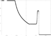
A movie (Figure 11![]() ) shows the Problem 2 blast wave evolution obtained with the relativistic PPM
method introduced in Section 3.1) on a grid of 2000 equidistant zones. At this resolution the relativistic
PPM code obtains a converged solution. The method of Falle and Komissarov [89
) shows the Problem 2 blast wave evolution obtained with the relativistic PPM
method introduced in Section 3.1) on a grid of 2000 equidistant zones. At this resolution the relativistic
PPM code obtains a converged solution. The method of Falle and Komissarov [89![]() ] requires a seven level
adaptive grid calculation to achieve the same, the finest grid spacing corresponding to a grid of 3200 zones.
As their code is free of numerical diffusion and dispersion, Wen et al. [295
] requires a seven level
adaptive grid calculation to achieve the same, the finest grid spacing corresponding to a grid of 3200 zones.
As their code is free of numerical diffusion and dispersion, Wen et al. [295![]() ] are able to handle this
problem with high accuracy (see Figure 12
] are able to handle this
problem with high accuracy (see Figure 12![]() ). At lower resolution (400 zones) the relativistic
PPM method reaches only 69% of the theoretical shock compression value (54% in case of the
second-order accurate upwind method of Falle and Komissarov [89
). At lower resolution (400 zones) the relativistic
PPM method reaches only 69% of the theoretical shock compression value (54% in case of the
second-order accurate upwind method of Falle and Komissarov [89![]() ]; 60% with the code of Donat et
al. [75
]; 60% with the code of Donat et
al. [75![]() ]).
]).
Get Flash to see this player.
Chow and Monaghan [53![]() ] have considered Problem 2 to test their relativistic SPH code. Besides a 15%
overshoot in the shell’s density, the code produces a non-causal blast wave propagation speed (i.e.,
] have considered Problem 2 to test their relativistic SPH code. Besides a 15%
overshoot in the shell’s density, the code produces a non-causal blast wave propagation speed (i.e.,
![]() ).
).
Anninos and Fragile [10![]() ] have considered Problem 2 as a test case for their artificial-viscosity based,
explicit codes. They find a 40% overshoot in the shock density contrast. This demonstrates that the extra
coupling introduced in the equations when using a consistent formulation of the artificial viscosity requires
the usage of implicit algorithms.
] have considered Problem 2 as a test case for their artificial-viscosity based,
explicit codes. They find a 40% overshoot in the shock density contrast. This demonstrates that the extra
coupling introduced in the equations when using a consistent formulation of the artificial viscosity requires
the usage of implicit algorithms.
The collision of two strong blast waves was used by Woodward and Colella [300] to compare the
performance of several numerical methods in classical hydrodynamics. In the relativistic case, Yang et
al. [303] considered this problem to test the high-order extensions of the relativistic beam scheme, whereas
Martí and Müller [181![]() ] used it to evaluate the performance of their relativistic PPM code. In this last
case, the original boundary conditions were changed (from reflecting to outflow) to avoid the reflection
and subsequent interaction of rarefaction waves allowing for a comparison with an analytical
solution. In the following we summarize the results on this test obtained by Martí and Müller
in [181
] used it to evaluate the performance of their relativistic PPM code. In this last
case, the original boundary conditions were changed (from reflecting to outflow) to avoid the reflection
and subsequent interaction of rarefaction waves allowing for a comparison with an analytical
solution. In the following we summarize the results on this test obtained by Martí and Müller
in [181![]() ].
].
The initial data corresponding to this test, consisting of three constant states with large pressure jumps
at the discontinuities separating the states (at x = 0.1 and x = 0.9), as well as the properties of the blast
waves created by the decay of the initial discontinuities, are listed in Table 11. The propagation velocity of
the two blast waves is slower than in the Newtonian case, but very close to the speed of light (0.9776 and
–0.9274 for the shock wave propagating to the right and left, respectively). Hence, the shock interaction
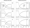
occurs later (at t = 0.420) than in the Newtonian problem (at t = 0.028). The top panel in Figure 13![]() shows four snapshots of the density distribution including the moment of the collision of the blast
waves at t = 0.420 and x = 0.5106. At the time of collision the two shells have a width of
shows four snapshots of the density distribution including the moment of the collision of the blast
waves at t = 0.420 and x = 0.5106. At the time of collision the two shells have a width of
![]() = 0.008 (left shell) and
= 0.008 (left shell) and ![]() = 0.019 (right shell), respectively, i.e., the entire interaction
takes place in a very thin region (about 10 times smaller than in the Newtonian case where
= 0.019 (right shell), respectively, i.e., the entire interaction
takes place in a very thin region (about 10 times smaller than in the Newtonian case where
![]() ).
).
| Left | Middle | Right | |||
| |
1000.00 | 0.01 | 100.00 | ||
| |
1.00 | 1.0 | 1.00 | ||
| |
0.00 | 0.00 | 0.00 | ||
| 0.957 | –0.882 | ||||
| 0.021 t | 0.045 t | ||||
| 0.978 | –0.927 | ||||
| 14.39 | 9.72 | ||||
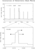
The collision gives rise to a narrow region of very high density (see lower panel of Figure 13![]() ) bounded
by two shocks moving at speeds 0.088 (shock at the left) and 0.703 (shock at the right) and large
compression ratios (7.26 and 12.06, respectively) well above the classical limit for strong shocks (6.0 for
) bounded
by two shocks moving at speeds 0.088 (shock at the left) and 0.703 (shock at the right) and large
compression ratios (7.26 and 12.06, respectively) well above the classical limit for strong shocks (6.0 for
![]() = 1.4). The solution just described applies until t = 0.430, when the next interaction takes
place.
= 1.4). The solution just described applies until t = 0.430, when the next interaction takes
place.
The complete analytical solution before and after the collision up to time t = 0.430 can be obtained
following Appendix II in [181![]() ].
].
Get Flash to see this player.
Get Flash to see this player.
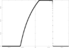
A movie (Figure 14![]() ) shows the evolution of the density up to the time of shock collision at t = 0.4200.
The movie was obtained with the relativistic PPM code of Martí and Müller [181
) shows the evolution of the density up to the time of shock collision at t = 0.4200.
The movie was obtained with the relativistic PPM code of Martí and Müller [181![]() ]. The presence of very
narrow structures involving large density jumps requires very fine zoning to resolve the states
properly. For the movie a grid of 4000 equidistant zones was used. The relative error in the
density of the left (right) shell is always less than 2.0% (0.6%), and is about 1.0% (0.5%) at the
moment of shock collision. Profiles obtained with the relativistic Godunov method (first-order
accurate, not shown) show relative errors in the density of the left (right) shell of about 50%
(16%) at t = 0.20. The errors drop only slightly to about 40% (5%) at the time of collision
(t = 0.420).
]. The presence of very
narrow structures involving large density jumps requires very fine zoning to resolve the states
properly. For the movie a grid of 4000 equidistant zones was used. The relative error in the
density of the left (right) shell is always less than 2.0% (0.6%), and is about 1.0% (0.5%) at the
moment of shock collision. Profiles obtained with the relativistic Godunov method (first-order
accurate, not shown) show relative errors in the density of the left (right) shell of about 50%
(16%) at t = 0.20. The errors drop only slightly to about 40% (5%) at the time of collision
(t = 0.420).
A movie (Figure 15![]() ) shows the numerical solution after the interaction has occurred. Compared to the
other movie (Figure 14
) shows the numerical solution after the interaction has occurred. Compared to the
other movie (Figure 14![]() ), a very different scaling for the x-axis had to be used to display the
narrow dense new states produced by the interaction. Obviously, the relativistic PPM code
resolves the structure of the collision region satisfactorily well, the maximum relative error in the
density distribution being less than 2.0%. When using the first-order accurate Godunov method
instead, the new states are strongly smeared out, and the positions of the leading shocks are
wrong.
), a very different scaling for the x-axis had to be used to display the
narrow dense new states produced by the interaction. Obviously, the relativistic PPM code
resolves the structure of the collision region satisfactorily well, the maximum relative error in the
density distribution being less than 2.0%. When using the first-order accurate Godunov method
instead, the new states are strongly smeared out, and the positions of the leading shocks are
wrong.
| http://www.livingreviews.org/lrr-2003-7 |
© Max Planck Society and the author(s)
Problems/comments to |