The solution to this problem is self-similar, because it only depends on the two constant states defining
the discontinuity ![]() and
and ![]() , where
, where ![]() , and on the ratio
, and on the ratio ![]() , where
, where
![]() and
and ![]() are the initial location of the discontinuity and the time of breakup, respectively. Both in
relativistic and classical hydrodynamics the discontinuity decays into two elementary nonlinear waves
(shocks or rarefactions) which move in opposite directions towards the initial left and right states. Between
these waves two new constant states
are the initial location of the discontinuity and the time of breakup, respectively. Both in
relativistic and classical hydrodynamics the discontinuity decays into two elementary nonlinear waves
(shocks or rarefactions) which move in opposite directions towards the initial left and right states. Between
these waves two new constant states ![]() and
and ![]() (note that
(note that ![]() and
and ![]() in Figure 1
in Figure 1![]() ) appear, which are separated from each other by a contact discontinuity moving
with the fluid. Accordingly, the time evolution of a Riemann problem can be represented as
) appear, which are separated from each other by a contact discontinuity moving
with the fluid. Accordingly, the time evolution of a Riemann problem can be represented as
As in the Newtonian case, the compressive character of shock waves (density and pressure rise
across the shock) allows us to discriminate between shocks (![]() ) and rarefaction waves (
) and rarefaction waves (![]() ):
):
Across the contact discontinuity the density exhibits a jump, whereas pressure and normal velocity are
continuous (see Figure 1![]() ). As in the classical case, the self-similar character of the flow through rarefaction
waves and the Rankine–Hugoniot conditions across shocks provide the relations to link the
intermediate states
). As in the classical case, the self-similar character of the flow through rarefaction
waves and the Rankine–Hugoniot conditions across shocks provide the relations to link the
intermediate states ![]() (
(![]() ) with the corresponding initial states
) with the corresponding initial states ![]() . They also allow
one to express the normal fluid flow velocity in the intermediate states (
. They also allow
one to express the normal fluid flow velocity in the intermediate states (![]() for the case of
an initial discontinuity normal to the
for the case of
an initial discontinuity normal to the ![]() axis) as a function of the pressure
axis) as a function of the pressure ![]() in these
states.
in these
states.
The solution of the Riemann problem consists in finding the intermediate states ![]() and
and ![]() , as well
as the positions of the waves separating the four states (which only depend on
, as well
as the positions of the waves separating the four states (which only depend on ![]() ,
, ![]() ,
, ![]() , and
, and ![]() ).
The functions
).
The functions ![]() and
and ![]() allow one to determine the functions
allow one to determine the functions ![]() and
and ![]() , respectively.
The pressure
, respectively.
The pressure ![]() and the flow velocity
and the flow velocity ![]() in the intermediate states are then given by the condition
in the intermediate states are then given by the condition
In the case of relativistic hydrodynamics, the major difference to classical hydrodynamics stems from the role of tangential velocities. While in the classical case the decay of the initial discontinuity does not depend on the tangential velocity (which is constant across shock waves and rarefactions), in relativistic calculations the components of the flow velocity are coupled by the presence of the Lorentz factor in the equations. In addition, the specific enthalpy also couples with the tangential velocities, which becomes important in the thermodynamically ultrarelativistic regime.
The functions ![]() are defined by
are defined by
The fact that one Riemann invariant is constant across any rarefaction wave provides the relation
needed to derive the function ![]() . In differential form, the function reads
. In differential form, the function reads
Considering that in a Riemann problem the state ahead of the rarefaction wave is known, the integration
of Equation (19![]() ) allows one to connect the states ahead (
) allows one to connect the states ahead (![]() ) and behind the rarefaction wave. Moreover,
using Equation (21
) and behind the rarefaction wave. Moreover,
using Equation (21![]() ), the EOS, and the following relation obtained from the constraint
), the EOS, and the following relation obtained from the constraint ![]() ,
that holds across the rarefaction wave,
,
that holds across the rarefaction wave,
In the limit of zero tangential velocities, ![]() , the function g does not contribute. In this limit and in
the case of an ideal gas EOS one has
, the function g does not contribute. In this limit and in
the case of an ideal gas EOS one has
The family of all states ![]() , which can be connected through a shock with a given state
, which can be connected through a shock with a given state ![]() ahead
of the wave, is determined by the shock jump conditions. One obtains
ahead
of the wave, is determined by the shock jump conditions. One obtains
Finally, the tangential velocities in the post-shock states can be obtained from [235![]() ]
]
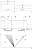
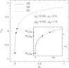
Figure 2![]() shows the solution of a particular mildly relativistic Riemann problem for different values of
the tangential velocity. The crossing point of any two lines in the upper panel gives the pressure and the
normal velocity in the intermediate states. The range of possible solutions in the (
shows the solution of a particular mildly relativistic Riemann problem for different values of
the tangential velocity. The crossing point of any two lines in the upper panel gives the pressure and the
normal velocity in the intermediate states. The range of possible solutions in the (![]() )-plane is marked
by the shaded region. While the pressure in the intermediate state can take any value between
)-plane is marked
by the shaded region. While the pressure in the intermediate state can take any value between ![]() and
and
![]() , the normal flow velocity can be arbitrarily close to zero in the case of an extremely relativistic
tangential flow. The values of the tangential velocity in the states
, the normal flow velocity can be arbitrarily close to zero in the case of an extremely relativistic
tangential flow. The values of the tangential velocity in the states ![]() and
and ![]() are obtained from the
value of the corresponding functions at
are obtained from the
value of the corresponding functions at ![]() in the lower panel of Figure 2
in the lower panel of Figure 2![]() . The influence of initial left
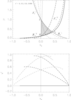
and right tangential velocities on the solution of a Riemann problem is enhanced in highly
relativistic problems. We have computed the solution of one such problem (see Section 6.2.2 below,
Problem 2) for different combinations of
. The influence of initial left
and right tangential velocities on the solution of a Riemann problem is enhanced in highly
relativistic problems. We have computed the solution of one such problem (see Section 6.2.2 below,
Problem 2) for different combinations of ![]() and
and ![]() . The initial data are
. The initial data are ![]() = 103,
= 103,
![]() = 1,
= 1, ![]() = 0;
= 0; ![]() = 10–2,
= 10–2, ![]() = 1,
= 1, ![]() = 0, and the 9 possible combinations of
= 0, and the 9 possible combinations of
![]() = 0, 0.9, 0.99. The results are given in Figure 3
= 0, 0.9, 0.99. The results are given in Figure 3![]() and Table 1, and a complete discussion can be
found in [235
and Table 1, and a complete discussion can be
found in [235![]() ].
].
| |
|
|
|
|
||||
| 0.00 | 0.00 | 9.16 × 10⁻² | 1.04 × 10+1 | 1.86 × 10+1 | 0.960 | 0.987 | –0.816 | +0.668 |
| 0.00 | 0.90 | 1.51 × 10 –1 | 1.46 × 10+1 | 4.28 × 10+1 | 0.913 | 0.973 | –0.816 | +0.379 |
| 0.00 | 0.99 | 2.89 × 10 –1 | 4.36 × 10+1 | 1.27 × 10+2 | 0.767 | 0.927 | –0.816 | –0.132 |
| 0.90 | 0.00 | 5.83 × 10⁻³ | 3.44 × 10+0 | 1.89 × 10⁻¹ | 0.328 | 0.452 | –0.525 | +0.308 |
| 0.90 | 0.90 | 1.49 × 10⁻² | 4.46 × 10+0 | 9.04 × 10⁻¹ | 0.319 | 0.445 | –0.525 | +0.282 |
| 0.90 | 0.99 | 5.72 × 10⁻² | 7.83 × 10+0 | 8.48 × 10+0 | 0.292 | 0.484 | –0.525 | +0.197 |
| 0.99 | 0.00 | 1.99 × 10⁻³ | 1.91 × 10+0 | 3.16 × 10⁻² | 0.099 | 0.208 | –0.196 | +0.096 |
| 0.99 | 0.90 | 3.80 × 10⁻³ | 2.90 × 10+0 | 9.27 × 10⁻² | 0.098 | 0.153 | –0.196 | +0.094 |
| 0.99 | 0.99 | 1.29 × 10⁻² | 4.29 × 10+0 | 7.06 × 10⁻¹ | 0.095 | 0.140 | –0.196 | +0.085 |
Finally, let us note that the procedure to obtain the pressure in the intermediate states ![]() is valid for
general EOS. Once
is valid for
general EOS. Once ![]() has been obtained, the remaining state quantities and the complete Riemann
solution,
has been obtained, the remaining state quantities and the complete Riemann
solution,
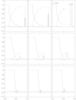
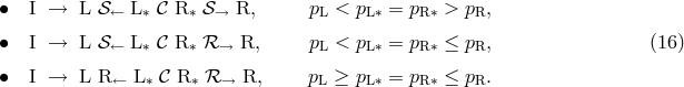
Solving a Riemann problem involves the solution of an algebraic equation for the pressure
(Equation (17![]() )). Moreover, the functional form of this equation depends on the wave pattern under
consideration (see expressions (16
)). Moreover, the functional form of this equation depends on the wave pattern under
consideration (see expressions (16![]() ). In a recent paper [241
). In a recent paper [241![]() ], Rezzolla and Zanotti have presented a
procedure, suitable for implementation into an exact Riemann solver in one dimension, which removes the
ambiguity arising from the wave pattern. That method exploits the fact that the expression for the relative
velocity between the two initial states is a (monotonic) function of the unknown pressure,
], Rezzolla and Zanotti have presented a
procedure, suitable for implementation into an exact Riemann solver in one dimension, which removes the
ambiguity arising from the wave pattern. That method exploits the fact that the expression for the relative
velocity between the two initial states is a (monotonic) function of the unknown pressure, ![]() , which
determines the wave pattern. Hence, comparing the value of the (special relativistic) relative velocity
between the initial left and right states with the values of the limiting relative velocities for the occurrence
of the wave patterns (16
, which
determines the wave pattern. Hence, comparing the value of the (special relativistic) relative velocity
between the initial left and right states with the values of the limiting relative velocities for the occurrence
of the wave patterns (16![]() ), one can determine a priori which of the three wave patterns will actually
result (see Figure 4
), one can determine a priori which of the three wave patterns will actually
result (see Figure 4![]() ). In [242] the authors extend the above procedure to multi-dimensional
flows.
). In [242] the authors extend the above procedure to multi-dimensional
flows.
| http://www.livingreviews.org/lrr-2003-7 |
© Max Planck Society and the author(s)
Problems/comments to |

![∘ -------------------------------- vx(1 − c2) ± c (1 − v2)[1 − v2c2− (vx)2(1 − c2)] ξ± = --------s-----s-----------------s-------------s-, (21 ) 1 − v2c2s](article105x.gif)