4 Apparatus and Principal Noise Sources
The detector consists of the earth and a spacecraft as separated test masses, electromagnetically-tracked using a precision Doppler system. The ground stations for the Doppler system are the antennas of the NASA/JPL Deep Space Network (DSN). Figure 3* shows DSS 25, the high-precision tracking station used in the Cassini gravitational-wave observations and other Cassini radio science investigations.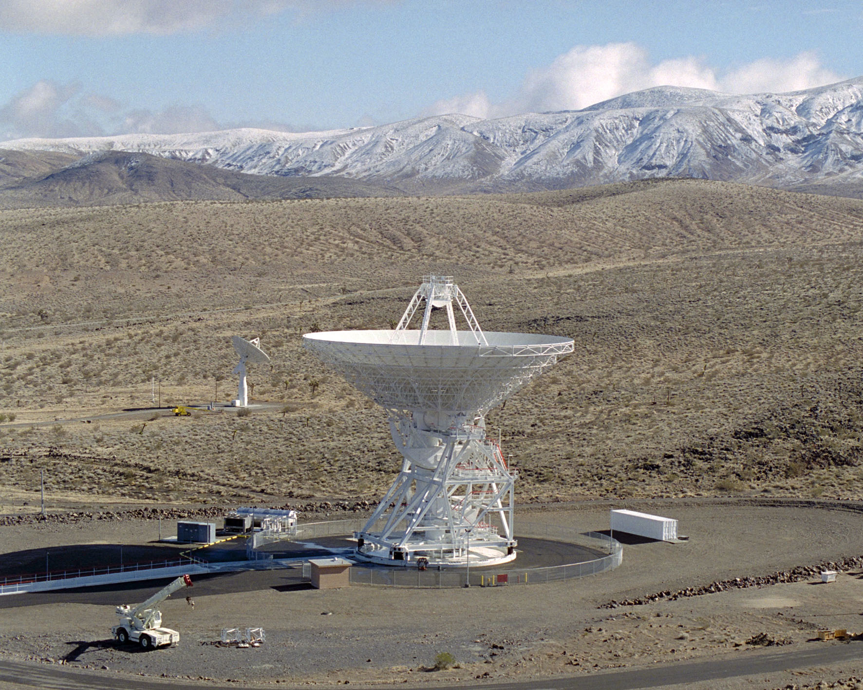
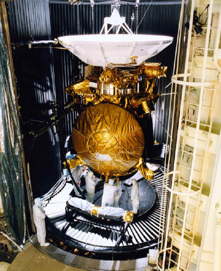
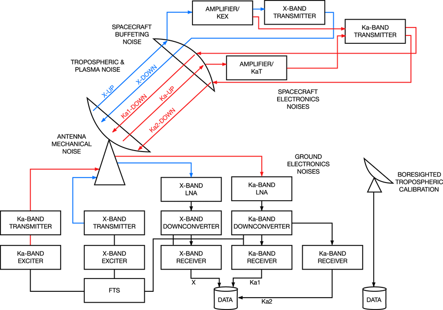
Figure 4* shows an example of the other part of the Doppler system. This is the Cassini spacecraft during ground tests. (Reference [37*] gives a popular discussion of the Cassini mission, the spacecraft, and its instrumentation.) The Doppler system is shown functionally in Figure 5*: A precision frequency standard from the Frequency and Timing Subsystem (FTS) provides the frequency reference to both the transmitter and receiver chains. On the transmitter side, the so-called exciter produces a near-monochromatic signal, referenced to the FTS signal but at the desired transmit frequency. This is amplified by the transmitter (with a closed-loop feedback system around the power amplifier to ensure frequency stability is not degraded) and routed via waveguide to the transmitter feedhorn in the basement of the antenna. (To correct for aberration the Ka-band transmit feed horn is on a table which is articulated in the horizontal plane. This allows the Ka-band transmitted beam to be pointed correctly relative to the received beam. The X-band feed is common to both the transmit and receive chains.) In a beam waveguide antenna the transmitted beam is reflected off of six mirrors within the antenna up to the subreflector (near the prime focus), then back to the main dish and out to the spacecraft (passing first through the troposphere, ionosphere, and solar wind). When the signal is received at the spacecraft it is amplified and phase-coherently re-transmitted to the earth. The received beam bounces off the main reflector to the subreflector and then, via mirrors and dichroic plates, to the receiver feed horn in the antenna basement. The received signal is downconverted to an intermediate frequency where it is digitized. The digital samples are processed to tune out the (very predictable) gross Doppler shift, and reduce the bandwidth of the samples. For GW operations, the bandwidth of the pre-detection data is typically reduced to 1 kHz, and those data are recorded to disk along with the tuning information. The phase of the signal is detected in software and, using the tuning information, the received sky frequency is reconstructed. This and the known frequency of the transmitted signal are used to compute the Doppler time series. Removal of the orbital signature and correction for charged particle and tropospheric scintillation gives Doppler residuals, which are used in subsequent processing steps to search for GWs (or for other radio science objectives [29*, 131*, 78*, 22*]).
Of course this cannot be done without introducing noise. The following Sections 4.1 – 4.11 summarize the principal noises, their spectra or Allan deviations3, and their transfer functions to the two-way Doppler time series.
4.1 Frequency standard noise
In two-way Doppler coherence is maintained by the frequency standard to which the up- and downlinks are referenced. Thus noise introduced by the frequency standard is of particular importance. Figure 6* shows fractional frequency stability as a function of integration time for several frequency standard technologies. In Cassini-era observations noise in the frequency and timing system (FTS) contributed less than 10–15 at 1000 s and, although fundamental, is not the leading noise source at the current level of sensitivity. (FTS stability required for future Doppler experiments is discussed in Section 7.)
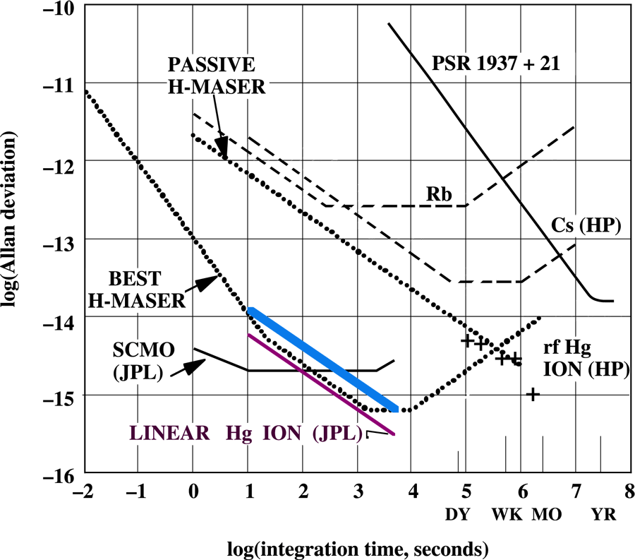
 (1000 s) less than 10–15. (Figure courtesy of
Lute Maleki; see also references [10*, 11*, 22*].)
(1000 s) less than 10–15. (Figure courtesy of
Lute Maleki; see also references [10*, 11*, 22*].) FTS noise enters the two-way Doppler time series via the transfer function [52*, 46*, 125*]
![yFTS (t) ∗ [δ(t) − δ(t − T2)]](article78x.gif) . The transfer functions of this and other principal noises are illustrated
schematically in Figure 7*. (An example of the FTS transfer function using real data is shown in Figure 8*.
Although the stability of the ground frequency standard is excellent, for a few days at the start of the first
Cassini Gravitational Wave Experiment there was an intermittent problem with an FTS distribution
amplifier at the Goldstone complex. The effect was to introduce isolated, fairly large, and very short glitches
into the frequency reference for both the transmitter and the receiver. This produced characteristic
anticorrelated glitches, separated by a two-way light time, in both the X- and Ka-band two-way Doppler
time series; see Figure 8*)
. The transfer functions of this and other principal noises are illustrated
schematically in Figure 7*. (An example of the FTS transfer function using real data is shown in Figure 8*.
Although the stability of the ground frequency standard is excellent, for a few days at the start of the first
Cassini Gravitational Wave Experiment there was an intermittent problem with an FTS distribution
amplifier at the Goldstone complex. The effect was to introduce isolated, fairly large, and very short glitches
into the frequency reference for both the transmitter and the receiver. This produced characteristic
anticorrelated glitches, separated by a two-way light time, in both the X- and Ka-band two-way Doppler
time series; see Figure 8*)
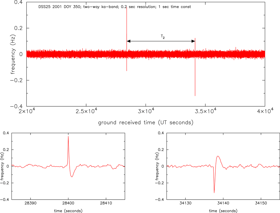
 1 s.
At this time resolution, the visual appearance of the time series is dominated by high-frequency noise.
Superimposed on this noise are two systematic glitches which were traced to an intermittently-faulty
distribution amplifier in the signal chain providing frequency references to the transmitter and
receiver. The distribution amplifier fault acts like an FTS glitch and, in the two-way Doppler, appears
twice in the time series anticorrelated at the two-way light time (Figure 7*). The glitches in the figure
are paired with the indicated two-way light time separation T2
1 s.
At this time resolution, the visual appearance of the time series is dominated by high-frequency noise.
Superimposed on this noise are two systematic glitches which were traced to an intermittently-faulty
distribution amplifier in the signal chain providing frequency references to the transmitter and
receiver. The distribution amplifier fault acts like an FTS glitch and, in the two-way Doppler, appears
twice in the time series anticorrelated at the two-way light time (Figure 7*). The glitches in the figure
are paired with the indicated two-way light time separation T2  5737.7 s. The lower panels show
blowups of the pair; the glitch waveforms are unresolved (shapes set by the impulse response of the
software phase detector) but clearly show the characteristic FTS anticorrelation.
5737.7 s. The lower panels show
blowups of the pair; the glitch waveforms are unresolved (shapes set by the impulse response of the
software phase detector) but clearly show the characteristic FTS anticorrelation.4.2 Plasma scintillation noise
The radio waves of the Doppler system pass through three irregular media: the troposphere, the ionosphere, and the
solar wind4.
Irregularities in the solar wind and ionospheric plasmas cause irregularities in the refractive index. The
refractive index fluctuations  for a cold unmagnetized plasma are
  and the
phase perturbation is
and the
phase perturbation is  , where
  is the wavelength,
  is the classical electron
radius, and
is the classical electron
radius, and  is the electron density fluctuation along the line of sight
  . These phase
perturbations mimic time-varying distance changes (thus velocity errors) and so are a noise source in
precision Doppler experiments. The transfer function of plasma phase scintillation to two-way
Doppler is shown schematically in Figure 7*. A solar wind plasma blob at a distance x from the
earth (producing a one-way fractional frequency fluctuation time series ysw) and an ionospheric
plasma blob at negligible light time from the ground station (with one-way time series yion)
produce two-way time series
. These phase
perturbations mimic time-varying distance changes (thus velocity errors) and so are a noise source in
precision Doppler experiments. The transfer function of plasma phase scintillation to two-way
Doppler is shown schematically in Figure 7*. A solar wind plasma blob at a distance x from the
earth (producing a one-way fractional frequency fluctuation time series ysw) and an ionospheric
plasma blob at negligible light time from the ground station (with one-way time series yion)
produce two-way time series ![sw y (t) ∗ [δ(t) + δ(t − T2 + 2x ∕c)]](article90x.gif) and
and ![ion y ∗ [δ(t) + δ(t − T2)]](article91x.gif) ,
respectively.
,
respectively.
 8021.5 s, indicating that the
features observed in the upper panels are caused by near-earth plasma.Update*
8021.5 s, indicating that the
features observed in the upper panels are caused by near-earth plasma.Update* (presumably ionospheric scintillation) and
  (localized solar wind
scintillation5)
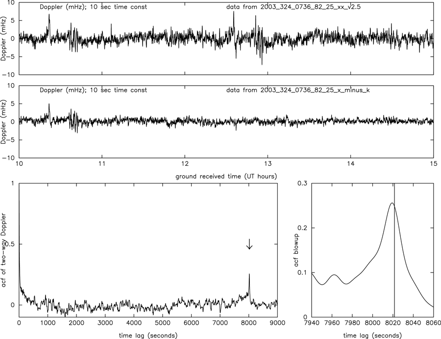
are shown in [9*]. Occasionally, however, large time-localized plasma events can be seen in the raw time
series. Figure 9* shows an example in Cassini data taken at DSS 25 on 2003 DOY 324. The top panel
shows the time series of the two-way X-band, with two discrete events observed near 10:20 and 10:40 ground
received time, echoed with positive correlation at about the two way light time. The middle
panel is the time series of X-(880/3344) Ka1Update*, which isolates the downlink plasma (and cancels
nondispersive processes such as FTS noise, tropospheric noise, antenna mechanical noise, and
gravitational waves; see Section 4.6). This indicates that the large events observed in the upper panel
are due to plasma scintillation. The lower panel shows the acf of the two-way Doppler time
series,
(localized solar wind
scintillation5)
are shown in [9*]. Occasionally, however, large time-localized plasma events can be seen in the raw time
series. Figure 9* shows an example in Cassini data taken at DSS 25 on 2003 DOY 324. The top panel
shows the time series of the two-way X-band, with two discrete events observed near 10:20 and 10:40 ground
received time, echoed with positive correlation at about the two way light time. The middle
panel is the time series of X-(880/3344) Ka1Update*, which isolates the downlink plasma (and cancels
nondispersive processes such as FTS noise, tropospheric noise, antenna mechanical noise, and
gravitational waves; see Section 4.6). This indicates that the large events observed in the upper panel
are due to plasma scintillation. The lower panel shows the acf of the two-way Doppler time
series, 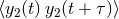 . The arrow marks the two-way light time. The acf peaks slightly earlier
than T2, indicating that the features observed in the other panels are caused by near-earth
plasma.
. The arrow marks the two-way light time. The acf peaks slightly earlier
than T2, indicating that the features observed in the other panels are caused by near-earth
plasma.
 ) at
) at  = 1000 s. S-band
  2.3 GHz; X-band
  8.4 GHz; Ka-band
 32 GHz. Red curves are for plasma scintillation at the indicated radio frequencies (circles are
S-band, more precisely: S-(3/11)X differential frequency fluctuations, data from Viking [131*, 21*]);
crosses are X-band (more precisely X-(880/3344) Ka1 differential frequency fluctuations, from
Cassini [122*, 11*, 19*, 29*, 121*]). Blue region shows typical uncalibrated tropospheric scintillation
levels at a moderate-altitude dry site such as Goldstone, CA, or the National Radio Astronomy
Observatory’s Very Large Array [20*, 75*, 76*]. Green arrows show upper (for antennas in the
DSN “high efficiency” sub-network, operated under operational but benign conditions) and
lower (for DSS 25, near solar opposition) limits to antenna mechanical noise [9*, 19*, 22*].
Update*Update*
32 GHz. Red curves are for plasma scintillation at the indicated radio frequencies (circles are
S-band, more precisely: S-(3/11)X differential frequency fluctuations, data from Viking [131*, 21*]);
crosses are X-band (more precisely X-(880/3344) Ka1 differential frequency fluctuations, from
Cassini [122*, 11*, 19*, 29*, 121*]). Blue region shows typical uncalibrated tropospheric scintillation
levels at a moderate-altitude dry site such as Goldstone, CA, or the National Radio Astronomy
Observatory’s Very Large Array [20*, 75*, 76*]. Green arrows show upper (for antennas in the
DSN “high efficiency” sub-network, operated under operational but benign conditions) and
lower (for DSS 25, near solar opposition) limits to antenna mechanical noise [9*, 19*, 22*].
Update*Update* Figure 10* summarizes the magnitude of the effect of plasma scintillation, tropospheric scintillation, and
antenna mechanical noise (the last two discussed below) on the stability of a Doppler tracking
system [46*, 9*, 10*, 11*, 12, 22*]. Shown in red are data and model curves for plasma phase scintillation:
Circles are S-band (frequency  2.3 GHz) observations taken in the ecliptic using the Viking orbiters
spacecraft taken over a wide range of sun-earth-spacecraft (SEP) angles [131, 21*]; crosses are X-band
(frequency
2.3 GHz) observations taken in the ecliptic using the Viking orbiters
spacecraft taken over a wide range of sun-earth-spacecraft (SEP) angles [131, 21*]; crosses are X-band
(frequency  8.4 GHz) taken near the antisolar direction using the Cassini spacecraft [19*, 22*]. Clearly
plasma scintillation minimizes for observations near the antisolar direction. The model curves drawn
through the data are described in [21*]. (Ionospheric phase scintillation is, of course, included in the data
presented in Figure 10*. Based on very limited multiple-station observations [21*] and on transfer
function studies [9*], high-elevation-angle plasma noise appears dominated by solar wind rather
than ionospheric phase scintillation. In any case, the effect of any plasma scintillation effect
can be made small by observing at high enough radio frequencies [128, 46*, 21] or by using
multi-link observations [65*, 41, 27, 122*, 121*, 29*] to solve-for and remove the plasma scintillation
effect.)
8.4 GHz) taken near the antisolar direction using the Cassini spacecraft [19*, 22*]. Clearly
plasma scintillation minimizes for observations near the antisolar direction. The model curves drawn
through the data are described in [21*]. (Ionospheric phase scintillation is, of course, included in the data
presented in Figure 10*. Based on very limited multiple-station observations [21*] and on transfer
function studies [9*], high-elevation-angle plasma noise appears dominated by solar wind rather
than ionospheric phase scintillation. In any case, the effect of any plasma scintillation effect
can be made small by observing at high enough radio frequencies [128, 46*, 21] or by using
multi-link observations [65*, 41, 27, 122*, 121*, 29*] to solve-for and remove the plasma scintillation
effect.)
4.3 Tropospheric scintillation noise
Phase fluctuations also arise from propagation through the neutral atmosphere. Here the so-called dry component of the troposphere is large but fairly steady with the wet component (water vapor fluctuations) being smaller but much more variable [20*, 95*, 94*, 96*, 76*]. Unlike plasma phase scintillation, propagation in the troposphere is effectively non-dispersive at microwave frequencies [71]. Figure 10* shows the magnitude of the effect: The blue cross-hatched region is the approximate level of uncalibrated tropospheric scintillation at NASA’s Goldstone Deep Space Communications Complex [75*]. Roughly, tropospheric scintillation is worse in the summer daytime and better on winter nights. Usually its raw magnitude is large compared with, e.g., antenna mechanical noise (discussed below.)
Experiments by George Resch and colleagues [95, 94*, 96*] were influential in showing that suitably
boresighted water vapor radiometer measurements could calibrate and remove much of the tropospheric
scintillation noise in both radioastronomical and precision spacecraft Doppler tracking observations. A
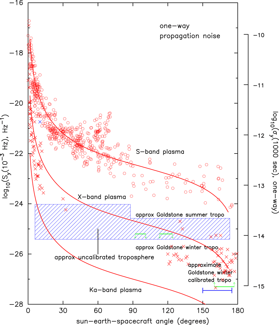
water-vapor-radiometer-based Advanced Media Calibration (AMC) system (Figure 11*) was developed and
installed near DSS 25 to provide tropospheric corrections for Cassini radio science observations. The AMC
system [94*, 96*, 76*] consists of two identical units placed close enough to each other and to DSS 25 that
the coherence of the tropospheric signal on the time scales of interest was high in all three time series
(see [10*, 11*] for examples of the squared-coherence as a function of Fourier frequency). The AMC
calibrations were used successfully in both the Cassini gravitational-wave observations [19*] and in relativity
and plasma experiments taken near solar conjunction [29*, 122*, 121*, 22*]. The transfer function of
tropospheric scintillation to the two-way Doppler is ![tropo y ∗ [δ(t) + δ(t − T2)]](article107x.gif) . Examples of the cross
correlation function of Doppler and the AMC-estimated tropospheric scintillation are shown
in [10, 11*].
. Examples of the cross
correlation function of Doppler and the AMC-estimated tropospheric scintillation are shown
in [10, 11*].
4.4 Antenna mechanical noise
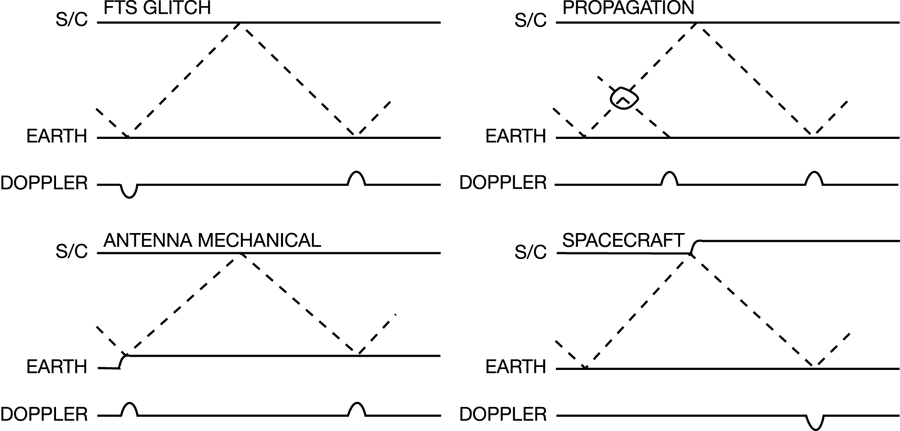
Figure 7* shows schematically how mechanical noise in the antenna enters the Doppler. If, for example, the
antenna’s phase center suddenly moves toward the spacecraft, the received signal is blue shifted, causing an
immediate effect in the Doppler. The motion also causes the transmitted signal to be blue shifted; this signal is
echoed in the time series a two-way light time later. Early tests by Otoshi and colleagues [86, 87] indicated
that antenna mechanical stability would contribute  10–15 for 1000 s integrations on a 34-m-class
antenna.6
10–15 for 1000 s integrations on a 34-m-class
antenna.6
Examples of the temporal autocorrelation of a typical Cassini DSS 25 Ka-band up- and downlink tracks
taken during the first Cassini GWE campaign in 2001 are shown in [19*, 11*]. Positive correlation at the
two-way light time is characteristic of low-level residual antenna mechanical noise and is observed (with
varying level of correlation at  = T2) in all the Cassini DSS 25 GW tracks. Antenna mechanical noise
in this band (
= T2) in all the Cassini DSS 25 GW tracks. Antenna mechanical noise
in this band ( 10–4 – 10–1 Hz) is thought to be caused by high-spatial-frequency irregularities in the
azimuth ring on which the antenna rolls, wind loading of the main dish, and uncorrected dish sag as the
elevation angle changes. In addition to this low-level statistical antenna mechanical noise, discrete events
positively correlated at the two-way light time and large enough to be visible by eye in the time
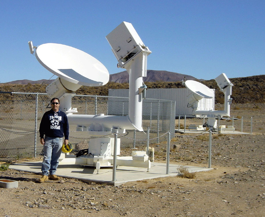
series are (rarely) observed in operational tracks [11*]. Figure 12* shows an example (Cassini
tracked by DSS 25 on 2001 DOY 330). The upper panel shows two-way Ka-band Doppler
residuals with approximately 10 s time resolution. The middle panel shows the time series of
X-(880/3344) Ka1, i.e., essentially the X-band plasma on the downlink, indicating the low level of plasma
noise on this day. The AMC data (not plotted here) similarly show low tropospheric noise.
The event at about 07:30 UT is echoed about a two-way light time later, and may be due to
gusting wind on this day (another candidate pair is at about 09:45 UT and a two-way light time
later). The lower panel shows the autocorrelation of the two-way Ka-band data, peaking at
T2.
10–4 – 10–1 Hz) is thought to be caused by high-spatial-frequency irregularities in the
azimuth ring on which the antenna rolls, wind loading of the main dish, and uncorrected dish sag as the
elevation angle changes. In addition to this low-level statistical antenna mechanical noise, discrete events
positively correlated at the two-way light time and large enough to be visible by eye in the time
series are (rarely) observed in operational tracks [11*]. Figure 12* shows an example (Cassini
tracked by DSS 25 on 2001 DOY 330). The upper panel shows two-way Ka-band Doppler
residuals with approximately 10 s time resolution. The middle panel shows the time series of
X-(880/3344) Ka1, i.e., essentially the X-band plasma on the downlink, indicating the low level of plasma
noise on this day. The AMC data (not plotted here) similarly show low tropospheric noise.
The event at about 07:30 UT is echoed about a two-way light time later, and may be due to
gusting wind on this day (another candidate pair is at about 09:45 UT and a two-way light time
later). The lower panel shows the autocorrelation of the two-way Ka-band data, peaking at
T2.
 5717.9 s. The lower right panel is a blow-up of the acf near the lag of a
two-way light time (indicated by the vertical line).
5717.9 s. The lower right panel is a blow-up of the acf near the lag of a
two-way light time (indicated by the vertical line). At lower Fourier frequencies (less than about 10–4 Hz) the apparatus operates in the LWL and the
signature of antenna mechanical noise is lost [19*]. At these low frequencies aggregate antenna
mechanical noise is probably composed both of approximately random processes (e.g., atmospheric
pressure loading of the station [81, 123, 38], differential thermal expansion of the structure [100*])
and of low-level quasi-deterministic processes (e.g., low-spatial-frequency imperfections in the
antenna’s azimuth track, systematic errors in subreflector focusing, etc.). Thermal processes (e.g.,
response of the structure to  10 K temperature variations during a track) can plausibly
produce only several millimeters of radio path length variation. The subreflector is continuously
repositioned to approximately compensate for elevation-angle dependent antenna distortions;
systematic errors in this focusing at the several millimeter level over the course of a track are
not unreasonable. Additionally, there are systematic low- and high-spatial-frequency height
variations,
10 K temperature variations during a track) can plausibly
produce only several millimeters of radio path length variation. The subreflector is continuously
repositioned to approximately compensate for elevation-angle dependent antenna distortions;
systematic errors in this focusing at the several millimeter level over the course of a track are
not unreasonable. Additionally, there are systematic low- and high-spatial-frequency height
variations,  6 mm peak-to-peak, in the azimuth track which will cause path-length variability.
Independently determined VLBI error budgets (omitting components due to radio source structure,
uncalibrated troposphere, and charged particle scintillation which are not common with Cassini-class
Doppler tracking observations) are believed dominated by station position and slowly-varying
antenna mechanical noises. These account for
6 mm peak-to-peak, in the azimuth track which will cause path-length variability.
Independently determined VLBI error budgets (omitting components due to radio source structure,
uncalibrated troposphere, and charged particle scintillation which are not common with Cassini-class
Doppler tracking observations) are believed dominated by station position and slowly-varying
antenna mechanical noises. These account for  1.3 cm rms path delay [104], occur on time
scales
1.3 cm rms path delay [104], occur on time
scales  10super5 – 106 s, and correspond to fractional frequency fluctuations
  10–15 or
smaller.
10–15 or
smaller.
4.5 Ground electronics noise
The DSN ground electronics have been carefully designed to minimize phase/frequency noise and
produce only a small contribution to the overall error budget. (Here I distinguish this noise
from the white phase noise due to finite signal-to-noise ratio; see Section 4.7). In a controlled
test at DSS 25 (antenna stationary, FTS common to the transmit and received chains and
thus cancelled in this zero two-way light time test) the sum of the noises from the exciter,
transmitter, downconversion electronics, and receiver was measured (Figure 5*). The power
spectrum of those test data is shown in [1*]; the corresponding Allan deviation at  = 1000 s is
2 × 10–16.
= 1000 s is
2 × 10–16.
4.6 Spacecraft transponder noise
Transponders accept an input carrier signal and produce an output signal at a different frequency. The process
is phase-coherent; that is, for every N integer cycles of the input there are M integer cycles of the output
(with M/N being the transponding ratio). When this condition is achieved, the transponder is operating
normally and produces an output that is “locked” to the input signal. The Cassini spacecraft has two
transponders7.
The standard flight transponder (“KEX”) accepts the X-band uplink and produces two phase-coherent
outputs, one at fX  880/749 (= X-band downlink frequency) and another at fX
  3344/749 (= Ka1
downlink frequency), where fX is the frequency of the X-band uplink signal observed at the spacecraft.
These signals are amplified, routed to the spacecraft high-gain antenna, and transmitted to the earth.
Another flight unit, the Ka-band Translator (“KaT”), accepts a Ka-band uplink signal and produces a
phase coherent signal with frequency fk
3344/749 (= Ka1
downlink frequency), where fX is the frequency of the X-band uplink signal observed at the spacecraft.
These signals are amplified, routed to the spacecraft high-gain antenna, and transmitted to the earth.
Another flight unit, the Ka-band Translator (“KaT”), accepts a Ka-band uplink signal and produces a
phase coherent signal with frequency fk  14/15 (= Ka2 downlink frequency), where fk is the Ka-band
signal frequency observed at the spacecraft.
14/15 (= Ka2 downlink frequency), where fk is the Ka-band
signal frequency observed at the spacecraft.
Pre-launch test data of transponders similar in design to Cassini’s KEX showed negligible (i.e., < 10–15)
frequency noise. Prelaunch tests of the KaT similarly showed negligible frequency noise ( 10–16 at
 = 1000 s), provided the received Ka-band uplink signal was relatively strong (greater than about
–127 dBm, see [1*, 19*, 78*, 22*]) at the input to the KaT.
= 1000 s), provided the received Ka-band uplink signal was relatively strong (greater than about
–127 dBm, see [1*, 19*, 78*, 22*]) at the input to the KaT.
Appropriate linear combinations of the frequency time series of the three downlinks can be used to estimate and remove (at the Fourier frequencies of interest) downlink and round-trip plasma noise [68, 65, 69*, 70*] in GW observations. For example, the downlink plasma noise time series can be determined by forming fX-(880/3344) fKa1, which is independent of FTS noise, antenna mechanical noise, spacecraft buffeting, and GWs (since these are all nondispersive.) These plasma corrections were also used with good success by Bertotti, Iess, and Tortora [29*] in a precision test of relativistic gravity involving Cassini tracking very close to the sun.
4.7 Thermal noise in the ground and spacecraft receivers
Finite signal-to-noise ratios in the up- and downlinks cause white phase noise. For observations to date, the
signal-to-noise ratio (SNR) of the downlink dominates. The one-sided spectral density of phase fluctuations
due to finite SNR,  , is
, is  1 / (SNR in 1 Hz band) rad2 Hz–1. The associated Allan deviation [23*]
is
1 / (SNR in 1 Hz band) rad2 Hz–1. The associated Allan deviation [23*]
is 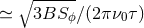 , where
  is the bandwidth of the detection system and assuming
  .
For Cassini gravitational wave observations, B is typically
.
For Cassini gravitational wave observations, B is typically  1 Hz and the typical X- or
Ka-band SNR in a 1 Hz bandwidth can be 45 dB or more. At
1 Hz and the typical X- or
Ka-band SNR in a 1 Hz bandwidth can be 45 dB or more. At  = 1000 s finite link SNR
contributes negligibly to the overall noise budget in current generation Doppler experiments (see
Table 2).
= 1000 s finite link SNR
contributes negligibly to the overall noise budget in current generation Doppler experiments (see
Table 2).
4.8 Spacecraft unmodeled motion
Unmodeled motion of the spacecraft enters directly into the two-way Doppler time series (see Figure 7*). The lack of a time-domain signature makes it difficult to isolate spacecraft motion using the Doppler data only. Such unmodeled motion can arise in principle from a variety of causes: fluctuations in the solar wind hitting the spacecraft, fluctuations in solar radiation pressure, physical articulation of spacecraft parts, leaking thrusters, sloshing of fuel in the spacecraft’s tanks, etc. Solar wind and solar radiation pressure fluctuations are computed to be far too small to affect observations at current levels of sensitivity [100*]. Articulation of instruments is restricted during quiet spacecraft periods where good Doppler sensitivity is required. Leaking thrusters and fuel sloshing are also thought to be small effects at current generation Doppler sensitivity [100].
In one case the as-flown spacecraft motion noise was independently determined. Using telemetry from
Cassini’s reaction wheel assembly, Won, Hanover, Belenky, and Lee [129*] inferred the time series of antenna
phase center motion projected onto the earth-spacecraft line (i.e., the sensitive axis for the Doppler system).
This test was done when Cassini was in semi-quiet cruise (thrusters off but with physical articulation of
elements of one science instrument, the Cassini Plasma Spectrometer, at  0.0025 Hz) for 40 hours
during 2001 DOY 152-153. The resulting Allan deviation for unmodeled spacecraft motion at
0.0025 Hz) for 40 hours
during 2001 DOY 152-153. The resulting Allan deviation for unmodeled spacecraft motion at
 = 1000 s was computed to be 2.3 × 10⁻¹⁶. Figure 13* shows the spectrum of velocity noise observed
in that test. Unmodeled motion of the spacecraft – at least the Cassini spacecraft – is thus negligible
compared with other noises at the sensitivity of current-generation Doppler experiments (see Figure 10* and
Table 2).
= 1000 s was computed to be 2.3 × 10⁻¹⁶. Figure 13* shows the spectrum of velocity noise observed
in that test. Unmodeled motion of the spacecraft – at least the Cassini spacecraft – is thus negligible
compared with other noises at the sensitivity of current-generation Doppler experiments (see Figure 10* and
Table 2).
4.9 Numerical noise in orbit removal
Update* Removal of the systematic variation in the Doppler time series due to the known motion of the earth and spacecraft can be done using the JPL/NASA Orbit Determination Program (ODP; [85]) or its successor the Mission-analysis, Operations, and Navigation Tool Environment (MONTE). Subtraction of the computed systematic Doppler frequency from the observed time series then gives residuals which can be searched for gravitational waves. The ODP computes Doppler by differencing the computed range to the spacecraft at two separated times and dividing by the time difference. Because of finite computer word length neither range nor time is expressed with perfect accuracy. These, coupled with finite-accuracy computer arithmetic, give rise to numerical noise which propagates to the residuals. Because of the granularity in time and distance the magnitude of numerical noise depends on time past 12:00 UT January 1, 2000 (the ODP measures time from J2000), distance and relative radial velocity of the spacecraft [133*] and is small compared with other noises for the early 2000s Cassini gravitational-wave observations (thus not included in Table 2). However, it is clear in Cassini Doppler data taken later in the Saturn tour [133, 67] and likely relevant for future, e.g., Juno and BepiColombo, observations.
4.10 Aggregate spectrum
Figure 14* shows the two-sided power spectrum of two-way fractional Doppler frequency, Sy2(f), computed from data taken at DSS 25 during the 2001 – 2002 solar opposition (from [19*]). It is derived after using the multi-link plasma corrections and the AMC tropospheric calibrations. The intrinsic frequency resolution of the spectrum is about 3 × 10⁻⁷ Hz. The spectrum in Figure 14* is smoothed to a resolution bandwidth of 3 × 10⁻⁶ Hz to reduce estimation error. Approximate 95% confidence limits for the logarithm of an individual smoothed spectral estimate are indicated [73*, 89*].
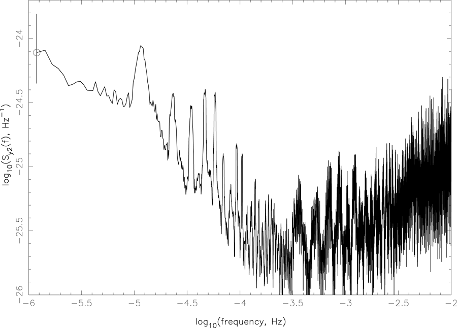
 3
3  Hz to reduce estimation error. Representative 95% confidence limits are indicated.
 The low-frequency part of the spectrum in Figure 14* consists of a continuum plus spectral lines between
 10–5 – 10–4 Hz. The lines in the unsmoothed spectrum are near the resolution limit of the 40 day
observation; their apparent width in Figure 14* is due to the spectral smoothing used to reduced estimation
error. The lowest frequency line is near one cycle/day; the other lines are near harmonics of one cycle/day.
Because of the multi-link plasma correction, all random processes contributing to this spectrum are
non-dispersive. At frequencies greater than about 1/T2 there is clear, approximately cosinusoidal,
modulation. This is characteristic of positive correlation in the time series at lag
10–5 – 10–4 Hz. The lines in the unsmoothed spectrum are near the resolution limit of the 40 day
observation; their apparent width in Figure 14* is due to the spectral smoothing used to reduced estimation
error. The lowest frequency line is near one cycle/day; the other lines are near harmonics of one cycle/day.
Because of the multi-link plasma correction, all random processes contributing to this spectrum are
non-dispersive. At frequencies greater than about 1/T2 there is clear, approximately cosinusoidal,
modulation. This is characteristic of positive correlation in the time series at lag  = T2, i.e., either
antenna mechanical noise or residual tropospheric noise. The level is too large to be dominated by residual
tropospheric scintillation, however, and so is interpreted as mechanical noise. Many minima of the
mechanical noise transfer function – at odd multiples of 1/(2 T2) – are easily visible in Figure 14*. The
spectrum appears to continue to be dominated by mechanical noise up to
= T2, i.e., either
antenna mechanical noise or residual tropospheric noise. The level is too large to be dominated by residual
tropospheric scintillation, however, and so is interpreted as mechanical noise. Many minima of the
mechanical noise transfer function – at odd multiples of 1/(2 T2) – are easily visible in Figure 14*. The
spectrum appears to continue to be dominated by mechanical noise up to  0.01 Hz, with the
signature of the transfer function being, however, difficult to see on this log plot (and also blurred
at high frequencies since T2 changed with time by about 3% over the course of the 40 day
observation.)
0.01 Hz, with the
signature of the transfer function being, however, difficult to see on this log plot (and also blurred
at high frequencies since T2 changed with time by about 3% over the course of the 40 day
observation.)
4.11 Summary of noise levels and transfer functions
To summarize the noise model: The principal noises are frequency and timing noise (FTS), plasma scintillation (solar wind and ionosphere), spacecraft electronics, unmodeled spacecraft motion, unmodeled ground antenna motion, tropospheric scintillation, ground electronics noise, thermal noise in the receiver, and systematic effects. The magnitudes of these noises in Cassini-era (2001 – 2008) observations are given in Table 2. Before any corrections, these noises enter the two-way Doppler as
where x is the effective distance of the solar wind perturbation from the earth. After multi-link plasma calibration, phase scintillation due to charged particles is effectively removed. Water-vapor-radiometer-based tropospheric calibration removes![noise FTS sw y2 (t) = y (t) ∗ [δ(t) − δ(t − T2)] + y (t) ∗ [δ(t) + δ(t − T2 + 2x∕c)] + yion ∗ [δ(t) + δ(t − T2 )] + ys∕c elect(t) ∗ δ(t − T2 ∕2) + ys∕c motion ∗ δ(t − T2 ∕2) + ant tropo ground elect y (t) ∗ [δ(t) + δ (t − T2)] + y (t) ∗ [δ(t) + δ(t − T2)] + y (t) + yrcvr + ysystematic(t), (4 )](article140x.gif)
 90% of the low-frequency fluctuations due to the neutral atmosphere,
so that the calibrated time series y2 is approximately
where
90% of the low-frequency fluctuations due to the neutral atmosphere,
so that the calibrated time series y2 is approximately
where ![gw y2(t) ≃ y2 + yFTS (t) ∗ [δ(t) − δ(t − T2)] + ys∕c elect(t) ∗ δ(t − T2∕2 ) + ys∕c motion ∗ δ(t − T ∕2 ) + yant(t) ∗ [δ(t) + δ (t − T )] + ytropo(t)∕10 ∗ [δ(t) + δ(t − T )] + ground elect r2cvr systematic 2 2 y (t) + y + y (t) = ygw + yother(t), (5 ) 2 2](article142x.gif)
 is all the non-GW (noise plus systematics) contributions to the two-way Doppler
variability.
is all the non-GW (noise plus systematics) contributions to the two-way Doppler
variability.
Table 2 summarizes the noise model and the associated Allan deviation at  = 1000 s for the
principal noises (models of the spectra of the individual noises are given in [111*]). Figure 5* shows, highly
schematically, the signal flow. This sketch, the GW transfer function (see Eq. (1*)), and the noise transfer
functions (see, e.g., Figure 7*) are used in discussions of sensitivity, signal processing, and for
qualifying/disqualifying candidate GW events.
= 1000 s for the
principal noises (models of the spectra of the individual noises are given in [111*]). Figure 5* shows, highly
schematically, the signal flow. This sketch, the GW transfer function (see Eq. (1*)), and the noise transfer
functions (see, e.g., Figure 7*) are used in discussions of sensitivity, signal processing, and for
qualifying/disqualifying candidate GW events.
|
Noise source |
|
Comment |
|
Frequency standard |
|
|
|
Antenna mechanical |
|
|
|
Ground electronics |
|
|
|
Plasma phase scintillation |
< 10–15, for Ka-band and SEP > 150° |
|
|
Stochastic spacecraft motion |
|
|
|
Receiver thermal noise |
few × 10–16 |
depends on link SNR and detector bandwidth [23] |
|
Spacecraft transponder noise |
|
|
|
Tropospheric
scintillation
|
< 3 × 10–15 to
|
|
|
Tropospheric
scintillation
|
< 1.5 × 10⁻¹⁵ to
|
under favorable conditions [19*]; median conditions in connected-element interferometry tests [96*] |
 [1000 s]
  8
8  2
2  2
2  depends
on SEP; dispersive; scales as
square of radio wavelength;
see Figure
depends
on SEP; dispersive; scales as
square of radio wavelength;
see Figure  2
2  10
10 30
30  3
3
 |
 |
 |