5 Signal Processing
This section discusses signal processing approaches, both formal and heuristic, which have been used to analyze Doppler observations. These include noise spectrum estimation, analysis methods to search for periodic, burst, and stochastic signals, and ideas for qualifying/disqualifying candidate signals based on signal and noise transfer functions.
5.1 Noise spectrum estimation
Spacecraft Doppler tracking shares attributes with all other real observations: The noise is non-stationary,
there are low-level systematic effects, and there are data gaps. The noise can usually be regarded as
effectively statistically stationary for at most the interval of a tracking pass ( 8 hours). The
non-stationarity of (what may be fundamentally Gaussian but with time-variable variance) noise is a
complication. For example in matched filtering for bursts, discussed below, the noise spectrum has to be
estimated locally [63*] for use in deriving locally-valid matching functions from the assumed GW
waveforms [61*].
8 hours). The
non-stationarity of (what may be fundamentally Gaussian but with time-variable variance) noise is a
complication. For example in matched filtering for bursts, discussed below, the noise spectrum has to be
estimated locally [63*] for use in deriving locally-valid matching functions from the assumed GW
waveforms [61*].
Noise characterization has historically been done via standard spectral and acf analysis techniques [73*]. Spectra of various data sets have been presented in [4*, 18*, 32*, 9*, 19*]. The data have typically been analyzed with varying time-frequency resolution to assess the fidelity of the spectral estimates and to provide local (in Fourier frequency) estimates of the underlying noise spectral density for sinusoidal and chirp signal searches (below). Running estimates of the variance and third central moments have been used as guides for identifying intervals of stationarity in pilot studies. Bispectra8 were computed for early data sets looking for non-linear, non-Gaussian effects. Bispectral analysis seemed to have limited utility, however; the Doppler noise is close to Gaussian and the slow convergence of higher statistical moments makes the bispectrum hard to estimate accurately over the length of a stationary data interval.
5.2 Sinusoidal and quasiperiodic waves
Some candidate sources radiate periodic or quasiperiodic waves. From an observational viewpoint a signal is
effectively a sinusoid if the change in wave frequency over the duration of the observation T is significantly
less than a resolution bandwidth 1/T. Since in a search experiment the signal phase is not known, spectral
analysis [73, 107*, 89*] is appropriate. In the absence of a signal, the real and imaginary parts of the time
series’ Fourier transform are Gaussian and uncorrelated, so the Fourier power is exponentially
distributed [88]. In the presence of a signal, the Fourier power is “Rice-squared” distributed [97*]. Formal
tests for statistical significance [55, 107, 4*, 18*, 7*, 5*, 89] involve comparing the power in a candidate line
with an estimate of the level of the local noise-spectrum continuum. Since the frequency of the
signal is also not known a priori, a range of frequencies must be searched. The spectral power is
approximately independent between Fourier bins, so the joint probability density function of the
power in  Fourier bins is the product of the individual bin pdfs. This can be used to set
statistical confidence limits for the sensitivity of a search experiment over multiple candidate signal
frequencies [18*].
Fourier bins is the product of the individual bin pdfs. This can be used to set
statistical confidence limits for the sensitivity of a search experiment over multiple candidate signal
frequencies [18*].
A signal is effectively a linear chirp if the change in frequency over the observation interval is > 1/T but
the curvature of the signal’s trajectory in a frequency-time plot is negligible over the observing interval. In
this case, signal power is smeared in (frequency, time) and simple spectral analysis is inappropriate. In a
chirp-wave analysis the Doppler data are first passed through a software preprocessor which tunes the signal
to compensate for the linear chirping. With the correct tuning function, the chirp is converted to a sinusoid
in the output. Spectral analysis is then used to search for statistically significant lines. The tuning function
 is complex. The parameter
  , an estimate of
  , is unknown and must be varied.
(In an idealized situation, this procedure resolves the signal into three lines, with frequency
separation depending on
, is unknown and must be varied.
(In an idealized situation, this procedure resolves the signal into three lines, with frequency
separation depending on  and T2 [5*]. The observability of all three lines is unlikely in real
observations, however.) The situation is different from the sinusoidal case in that an arrow
of time has been introduced by the software dechirping; the positive and negative frequency
components of the dechirped spectrum contain different information. In principle, an ensemble
of chirping signals, each too weak to be detected individually, could be identified by noting
differences in the statistics of the positive and negative frequency components of the dechirped
spectrum.
and T2 [5*]. The observability of all three lines is unlikely in real
observations, however.) The situation is different from the sinusoidal case in that an arrow
of time has been introduced by the software dechirping; the positive and negative frequency
components of the dechirped spectrum contain different information. In principle, an ensemble
of chirping signals, each too weak to be detected individually, could be identified by noting
differences in the statistics of the positive and negative frequency components of the dechirped
spectrum.
Waveforms which are more complicated than linear chirps arise, e.g., from binary systems near coalescence. To do proper matched filtering [61*] the waveform and the source location on the sky are needed. If one assumes the time evolution of the phase, the time series can be resampled at unequal times [102, 5*] so that (in terms of the resampled phase variable) the signal is periodic. This suboptimum technique can be used in pilot analyses to pre-qualify candidates for exact matched filtering. Nonsinusoidal periodic waves, generated, e.g., by non-circular binary systems, can have rich Fourier content [127*]. Searches for these waveforms have included folding the data with assumed periods [18*].
5.3 Bursts
Bursts are time-localized signals in the data set. Matched filtering with assumed waveforms involves varying
several parameters, including  , in the three-pulse response. Burst searches are helped by the very
diagnostic three-pulse response (integral of signal response must be zero; location and amplitude ratios of
the “pulses” must be consistent with
, in the three-pulse response. Burst searches are helped by the very
diagnostic three-pulse response (integral of signal response must be zero; location and amplitude ratios of
the “pulses” must be consistent with  .) Matched filter outputs have a “signal part” (integral of
the matching function with the signal) and a “noise part” (integral of the matching function
with the noise). The variance of the matched-filter’s noise-only output changes if the noise is
non-stationary. If not accounted for this can result in distorted pdfs of matched filter outputs and
(superficially significant) tails of the distribution of matched filter outputs, even in the absence
of a signal. To allow for this [63*] the data can be divided into intervals over which the noise
appears stationary. A model of the noise spectrum over each interval is used, along with the
assumed signal waveform, to compute the matching function. This matching function is then
used for that interval only. Simulation of the matched filter against synthetic noise having the
same spectrum and data gap structure of the interval being analyzed is used to estimate the
variance of the noise-only matched filter output. Then the actual matched filter outputs can be
normalized by the estimated noise-only variance to express outputs in terms of SNRs. This
allows the outputs of the matched filter to be compared consistently across a data set where
the noise statistics are changing. Multi-spacecraft coincidences can be used to reduce further
false-alarms [28*, 112*, 63*, 13*].
.) Matched filter outputs have a “signal part” (integral of
the matching function with the signal) and a “noise part” (integral of the matching function
with the noise). The variance of the matched-filter’s noise-only output changes if the noise is
non-stationary. If not accounted for this can result in distorted pdfs of matched filter outputs and
(superficially significant) tails of the distribution of matched filter outputs, even in the absence
of a signal. To allow for this [63*] the data can be divided into intervals over which the noise
appears stationary. A model of the noise spectrum over each interval is used, along with the
assumed signal waveform, to compute the matching function. This matching function is then
used for that interval only. Simulation of the matched filter against synthetic noise having the
same spectrum and data gap structure of the interval being analyzed is used to estimate the
variance of the noise-only matched filter output. Then the actual matched filter outputs can be
normalized by the estimated noise-only variance to express outputs in terms of SNRs. This
allows the outputs of the matched filter to be compared consistently across a data set where
the noise statistics are changing. Multi-spacecraft coincidences can be used to reduce further
false-alarms [28*, 112*, 63*, 13*].
Related to burst processing are “template independent” methods for identifying data intervals for more
detailed study. Wavelet transforms of the data on a pass-by-pass basis have been sometimes useful in finding
time-localized intervals formally contributing anomalously large variance. These are then typically checked
to see if there are corresponding features within  T2. Examination of the time series reconstructed from
some small fraction (
T2. Examination of the time series reconstructed from
some small fraction ( 10%) of the largest amplitude wavelets (or systematically from the wavelets in
selected subbands only) have also been useful [11*].
10%) of the largest amplitude wavelets (or systematically from the wavelets in
selected subbands only) have also been useful [11*].
5.4 Stochastic background
Stochastic background limits can be derived from the smoothed Doppler frequency power
spectrum [52*, 26*]. If the background is assumed isotropic, spectra of two-way Doppler can be
converted to spectra of strain by dividing by the sky- and polarization-averaged GW response
function [52*, 54*, 19*]. (If a background is not isotropic, then the spectral response function
is the square of the Fourier transform of the three-pulse response evaluated for the relevant
 and averaged over polarization states.) From Sh the strength of the background can be
expressed relative to closure density or as a characteristic strain amplitude [108*, 93*, 72*] (see
Section 6.5).
and averaged over polarization states.) From Sh the strength of the background can be
expressed relative to closure density or as a characteristic strain amplitude [108*, 93*, 72*] (see
Section 6.5).
5.5 Classification of data intervals based on transfer functions
Although the signal waveforms are not known a priori, there is a good understanding of transfer functions
of the GW signal and the principal noises to the Doppler. Partitioning the data into “known-noise-like” or
“other” intervals based on the noise transfer functions can be useful. Examples of discrete-event noise
classification based on transfer function were shown in Section 4; statistical classification of data intervals
based on the local acf is also possible (see, e.g., [9*, 19*]). The local spectrum or correlation function has also
been used to assess the relative importance of different noises and their stationarity from, e.g., the degree of
correlation at  = T2.
= T2.
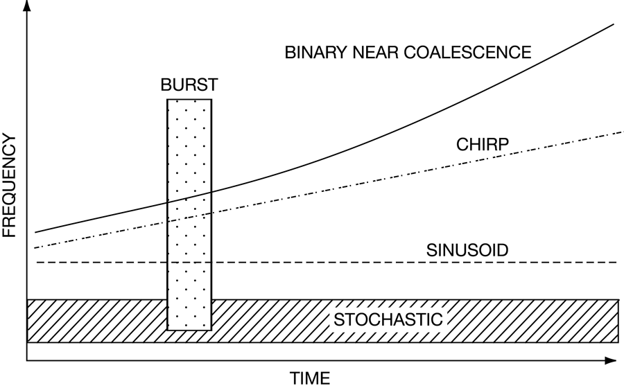
5.6 Frequency-time representations
It is often useful to think of signal representations in a frequency-time phase space, shown schematically in Figure 15*. There are many ways to tile frequency-time, e.g., Fourier transforms, wavelets, chirplets, Gabor-transforms (and variants, depending on the temporal windowing used); there is a correspondingly large literature. Depending on the situation each tiling can have special merit (e.g., if additional information suggests a specific candidate signal is likely to project preferentially onto a small fraction of a particular mathematical basis while the noise does not).
As an example, Figure 16* shows normalized Fourier power as a function of frequency-time for the Cassini two-way Ka-band track on 2001 DOY 350 (time series shown in Figure 8*). This plot was constructed by taking the unwindowed power spectrum of sequential 102.4 s data segments (in this case 75% overlapped in time). The heavy white line indicates the two-way light time at the beginning of the data set. The normalized power – power at a given (frequency, time) point divided by the estimated local continuum power near that point – is plotted. This is a nondimensional measure of the contrast (and potential statistical significance) of the Fourier power at that point relative to a local background. The color code runs from black (low values) through green to red (very high values). Points with estimated contrast ratio > 10 are marked with white circles. If two high-contrast features are at the same frequency and separated by a two-way light time, they are connected with a thin white line. The FTS glitch of Figure 8* is clearly evident in both the time series and in T2-separated bands of high-contrast Fourier power in the lower plot. Additional features not evident in the time series but paired at T2 are detected near the beginning of the data set and at low-frequency. See also Figures 17* and 18*.
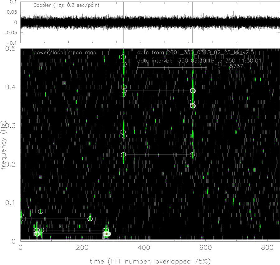
 1 s time constant, sampled at
0.2 s/sample. At this resolution the visual impression of the plot is set by relatively high frequency
noise. Lower right panel: low frequency resolution power spectrum of the full data set shown in
upper panel. Lower left panel: normalized dynamic spectrum of the data in the upper panel. This
was constructed by forming sequential spectra of short (
1 s time constant, sampled at
0.2 s/sample. At this resolution the visual impression of the plot is set by relatively high frequency
noise. Lower right panel: low frequency resolution power spectrum of the full data set shown in
upper panel. Lower left panel: normalized dynamic spectrum of the data in the upper panel. This
was constructed by forming sequential spectra of short ( 102 s) unwindowed segments of the
data. Each data segment is 75% overlapped with its neighbors. The heavy white line indicates the
two-way light time at the beginning of the data set. The plotted quantity is power at a given
point in (frequency-time) divided by a local estimate of the average power at that (frequency, time)
point, a nondimensional measure of the contrast of the Fourier power at that point relative to an
estimated background. The color code runs from black (low values) through green (higher values) to
red (very high values). Points with this estimated contrast ratio > 10 are marked with white circles.
If two high-contrast features are at the same frequency and separated by a two-way light time, they
are connected with a thin white line. The FTS glitch shown also in Figure 8* is clearly evident in
both the time series and in T2-separated bands of high-contrast Fourier power in the lower plot.
Additional features paired at T2 in the earlier, lower-frequency part of the data are also detected in
the normalized dynamic spectrum.
102 s) unwindowed segments of the
data. Each data segment is 75% overlapped with its neighbors. The heavy white line indicates the
two-way light time at the beginning of the data set. The plotted quantity is power at a given
point in (frequency-time) divided by a local estimate of the average power at that (frequency, time)
point, a nondimensional measure of the contrast of the Fourier power at that point relative to an
estimated background. The color code runs from black (low values) through green (higher values) to
red (very high values). Points with this estimated contrast ratio > 10 are marked with white circles.
If two high-contrast features are at the same frequency and separated by a two-way light time, they
are connected with a thin white line. The FTS glitch shown also in Figure 8* is clearly evident in
both the time series and in T2-separated bands of high-contrast Fourier power in the lower plot.
Additional features paired at T2 in the earlier, lower-frequency part of the data are also detected in
the normalized dynamic spectrum.5.7 Qualifying/disqualifying candidates
Qualifying or disqualifying candidate signals is based both on spectra of noise processes and, usually more crucially, on signal and noise transfer functions. In some cases it is immediately obvious, using the noise transfer function and a single time series, that a stretch of data is noise dominated (large antenna mechanical events for example). In other cases, multiple time series (e.g., the multiple X- and Ka-band signals available with the Cassini observations; see Figure 5*) can be used to qualify candidates.
As an example, candidate periodic and quasiperiodic signals have been disqualified in various data sets (discussed below) based on one or more of these considerations:
- Is there a radio wave amplitude variation associated with a Doppler variation (for GWs, there should not be)?
- Is there something special about the data taking or the data records where the candidate is
observed?
- Is the back-end instrumentation distinguished in some way (e.g., common receiver or receiver rack)?
- Is the candidate observed only at a specific tracking-station? (Is the candidate observed at only one kind of station, e.g., only at the DSN beam-waveguide antennas and not at the DSN “high-efficiency” antennas?)
- Is the signal a plausible alias of a man-made frequency?
- Could a narrow-band feature be due to a mechanical resonance of the antenna?
- Does it appear in only part(s) of the tracking record?
- Is its frequency modulation consistent with the source being at a fixed point on the sky, given the known earth-spacecraft geometry variation over the observation?
- Is the candidate observed in more than one radio band (e.g., X- and Ka-band) simultaneously? Is it
demonstrably non-dispersive? Are the individual-band SNRs consistent with a common
 v/c?
v/c?
- Is the candidate consistent when observed with different resolutions in time and Fourier frequency?
- Could this candidate have been introduced into the time series by a faulty calibration?
Each of the above has been used to assess reality or unreality of candidate periodic and quasiperiodic waves in different data sets. Some published examples include the following ones:
Anderson et al. [5*] observed a chirp that persisted over 10 days. The data were reanalyzed in subsets based on inclusion or exclusion of specific stations, specific transmitter/receiver pairs, and temporal partitions of the data set. The chirp was ultimately disqualified as non-astronomical because it was only observed in the subset of the data involving a particular transmitter/receiver pair.
In another Pioneer spacecraft observation [18*] the statistical significance of candidate spectral lines was assessed by scrambling the data within the data gaps and reanalyzing. This confirmed analytical work on the false alarm probability and the (lack of) statistical significance of the strongest candidate periodic signals.
In the three-spacecraft coincidence experiment involving the Galileo, Mars Observer, and Ulysses
spacecraft [13*] matched filtering for signals from particular directions that were sinusoidal (except for
modulation due to earth-spacecraft motion modulation over the course of the  20-day track) gave
undistinguished peak SNRs in the Mars Observer and Galileo data sets, but a formally significant SNR in
the Ulysses data set. From the modulation over the period of the observations, the inferred direction of
arrival was
20-day track) gave
undistinguished peak SNRs in the Mars Observer and Galileo data sets, but a formally significant SNR in
the Ulysses data set. From the modulation over the period of the observations, the inferred direction of
arrival was  ,
,  . Since the position of the candidate source was thus “known”,
gravitational-wave polarization states [127*, 18*, 16*] were explored looking for states which
could simultaneously couple well to Ulysses but poorly (so as to push a real astronomical signal
into the noise) to Mars Observer and Galileo. There was no polarization state which could
produce this simultaneously in the three data sets, so this candidate was excluded as a false
alarm.
. Since the position of the candidate source was thus “known”,
gravitational-wave polarization states [127*, 18*, 16*] were explored looking for states which
could simultaneously couple well to Ulysses but poorly (so as to push a real astronomical signal
into the noise) to Mars Observer and Galileo. There was no polarization state which could
produce this simultaneously in the three data sets, so this candidate was excluded as a false
alarm.
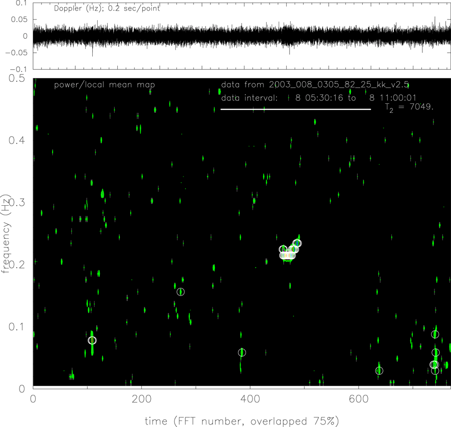
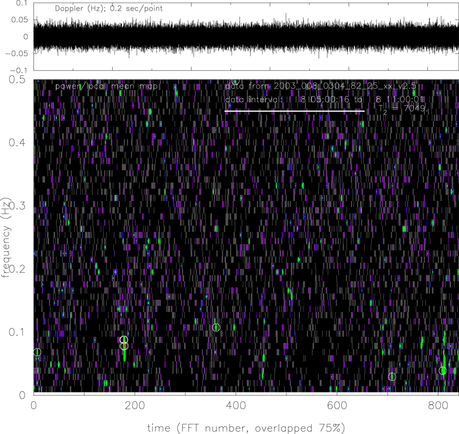
The consistency of multiple, simultaneous data sets can also be used to qualify or disqualify non-periodic waveform candidates. This is complicated by the fact that different data sets have different noise levels and thus different sensitivities to GWs. Figure 17* shows a normalized dynamic spectrum for Cassini two-way Ka-band data on 2003 DOY 008. The strong feature observed in the average spectrum (right panel) comes from a short time interval in the track at about 08:50 UT. Figure 18* shows the dynamic spectrum of two-way X-band for the same track, with no high-contrast feature near (08:50 UT, 0.22 Hz). Subsequent analysis of band pass filtered time series for the X- and Ka-band data showed that the event seen in the Ka-band data, if produced by a real earth-spacecraft velocity, should have also been observable above the noise in the X-band and was not. Such events were observed once per day in the 2002 – 2003 Cassini observing campaign (only – and with varying strength) and are apparently a systematic effect specific to the two-way Ka-band system (perhaps associated with the independence of the Ka-band transmit and receive horns; see Section 4.4 and Figure 5*).
Qualifying/disqualifying candidate burst waves is slightly different because, by hypothesis, the signal is only “on” for a finite time and some of the above tests do not apply. However a true GW burst must be nondispersive and show the correct three-pulse signature in the time series. Here the three-pulse response [52*] is very powerful: Whatever the GW waveforms, the signal must show the three-pulse response with correct amplitudes and spacings for a GW from a specific direction relative to the earth-spacecraft line (see Figure 1*).
5.8 Other comments
Another analysis scheme which is attractive in principle but does not seem useful in current-sensitivity Doppler data analysis is the Karhunen–Loéve expansion [61, 43]. This is a signal-independent approach where the data themselves are used to construct a mathematical basis to express the data. Such representations may be useful for template-free analysis of time series dominated by a signal of unknown waveform. However, experiments with this analysis procedure on simulated noise-dominated Doppler data sets were disappointing; the modes discovered in the Karhunen–Loéve simulations were always the noise modes.
Editing flags developed, e.g., from spacecraft telemetry or from DSN tracking logs have not historically been useful9 as veto signals (the internal monitoring capabilities of the spacecraft and ground stations were, of course, not intended for this purpose). The Doppler itself is much more sensitive than the system monitors and also – being spatially distributed by cT2 / 2 – has noise-signatures which often allow easier identification of specific disturbances affecting the time series (see, e.g., Section 4).
Even though each class of tracking antenna has a common design, there are low-level station-specific systematic differences. Getting data with different stations helps at least to identify these systematics (see, e.g., [5*]). Also data taken at low elevation angle (< 20°) with any antenna are statistically of poorer quality.
Finally, at current levels of sensitivity Doppler tracking observations are clearly search experiments. We are looking for signals with poorly-constrained waveforms which are “surprisingly” strong (thus expected to be rare). To maximize the chance that an unexpected real event will not be dismissed as due to a known noise process (or overlooked altogether), it is obviously useful to analyze the time series in different ways to bring out different aspects. Doppler tracking data sets are not impossibly large: It is practical for a person to actually look at all the data with varying time-frequency resolution – in addition to using formal and automated analysis procedures. (A potential difficulty is still actually recognizing unanticipated features if they are present. Reference [77] has interesting discussions of the problems of recognizing unexpected things.) As emphasized by Thorne [108*], the largest events may be from unexpected sources so the data analysis scheme must be robust enough that unexpected signals are not preprocessed away.
 |
 |
 |