6 Detector Performance
6.1 Observations to date
Table 3 lists spacecraft Doppler GW observations to date and observations possible in the near future. Update*
| Year | Spacecraft |
Comment |
Reference |
| 1980 | Voyager |
several passes; S-band uplink, S/X downlink; burst search |
[60*] |
| 1981 | Pioneer 10 |
3 passes; long T2; GW background limit; observationally excluded GW from Geminga |
[4*, 6*] |
| 1983 | Pioneer 11 |
3 days; long T2; broadband periodic search |
[18*] |
| 1988 | Pioneer 10 |
10 days; long T2; chirp wave search |
[5] |
| 1990 | Ulysses |
3.5 days; short T2 |
[31*, 32*] |
| 1992 | Ulysses |
14 days; long T2; periodic and chirp search; S-band uplink, S/X band downlink |
[31*, 32*] |
| 1993 | MO/GLL/ULS |
19 days; X/X-band on MO; coincidence experiment; search for all waveforms |
[63*, 64*, 13*] |
| 1994-5 | Galileo |
40/40 days (two oppositions); long T2; S/S-band |
[3*, 13*] |
| 1997 | MGS |
21 days; short T2; X/X-band |
[9*] |
| 2001-3 | Cassini |
40/40/20 days (three oppositions); long T2; Ka-band; AMC; multi-link plasma calibration |
[19*, 78] |
| 2016+ | Juno |
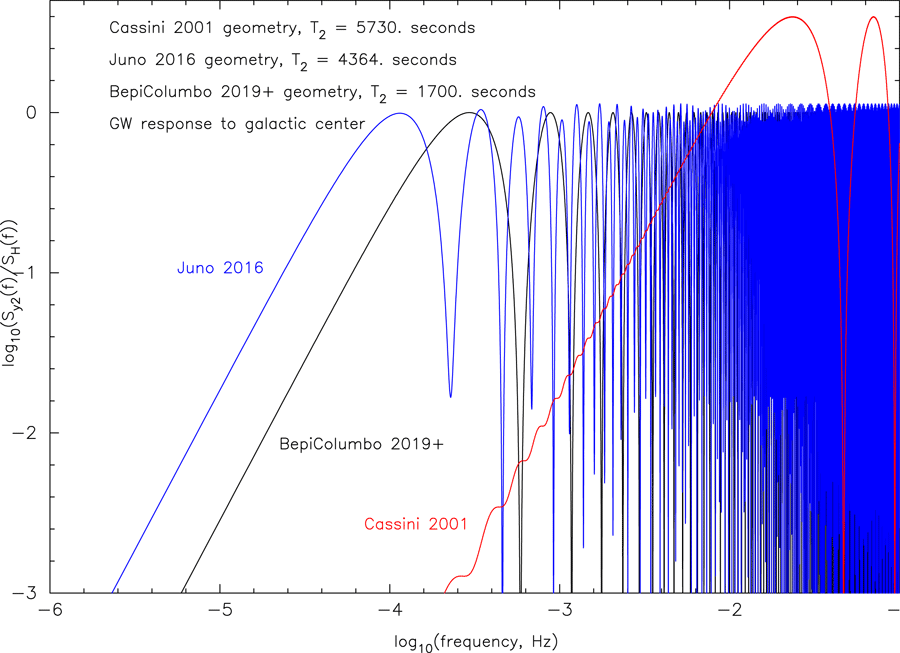
opposition in early 2016; long T2; Ka-band; AMC; good geometric coupling to galactic center |
[33, 83] |
| 2019+ | BepiColombo |
short T2; multi-link plasma calibration; AMC; good geometric coupling to galactic center |
[66, 25] |
The observations in Table 3 reflect increasing sensitivity between about 1980 and the early 2000s. These improvements were due both to engineering advancements (in spacecraft and in the DSN) and to programmatic decisions allowing use of planetary spacecraft for these observations. Voyager sensitivity was limited by a combination of plasma noise in the S-band uplink (see Figure 10*) and spacecraft buffeting noise from its thrusters. Although the data volume was small, those observations were used in the first formal search for low-frequency burst waves [60*]. The Pioneer spacecraft were spin-stabilized, resulting in lower spacecraft buffeting noise, but were again sensitivity-limited by plasma noise in the S-band radio links. Despite this, Pioneer data were able to observationally exclude putative sinusoidal GW emission from Geminga [4*] and place the then-best limit on a low-frequency GW background [6*]. Ulysses observations in 1992 were the longest to date, motivated innovations in signal processing, and resulted in the then-best sensitivity to periodic and chirp waveforms [31, 32*]. Mars Observer was the first spacecraft to have X-band on both the up- and downlinks, resulting in much-reduced plasma noise. Mars Observer, Galileo, and Ulysses did the first (and so far only) coincidence experiment [63*, 13*] which was used successfully to disqualify an event which was formally significant in one time series. Galileo observations in 1994 – 1995 had a long two-way light time and thus better GW response at lower Fourier frequencies. Unfortunately, the failure of the high-gain antenna required S-band only observations (thus high plasma noise) [9*]. Mars Global Surveyor observations in 1997 were done with X-band links (but off of solar opposition) and were the only observations where spacecraft engineering telemetry was used to correct the Doppler data for the (slow) systematic spacecraft motion. Those data also showed strong correlation at the two-way light time, indicating the importance of tropospheric calibration and placing upper limits on antenna mechanical noise [9*, 22].
Most of the sensitivity discussion in this paper, however, relates to Cassini observations. Cassini was launched on a mission to Saturn in 1997 [37]. After earth, Venus, and Jupiter gravity-assists, it continued on a free interplanetary cruise trajectory toward orbit insertion at Saturn. The Cassini gravitational-wave observations consisted of two 40-day data-taking campaigns, centered on the spacecraft’s solar oppositions during 2001 – 2002 and 2002 – 2003, and one 20-day observation taken somewhat off opposition during late 2003. This data set is distinguished by its very sophisticated multi-link radio system (allowing essentially perfect plasma correction [69, 122, 70, 29, 121]) and by the Advanced Media Calibration system (allowing excellent tropospheric scintillation removal) [94, 96, 19*, 76].
6.2 Near-future observations
Update* There are two potentially-good-sensitivity near-future GW opportunities using Juno and BepiColombo in their cruise phases. Juno will reach Jupiter in July 2016. BepiColombo is a low-altitude orbiter of Mercury.The Juno spacecraft has Ka-band up- and downlink, thus good immunity to plasma scintillation noise.
Juno’s two-way light time near opposition in 2016 will be about 4360 seconds, smaller than
that of Cassini (thus Juno will, in sky-average, have poorer low-frequency response). Juno is
distinguished, however, in that its GW coupling to the galactic center (the nearest plausible source
of strong millihertz GWs) is much better than that of Cassini. For Juno, near the 2016 solar
opposition, the cosine of the angle between the earth-spacecraft vector and the wavevector
for a source at the galactic center is  =
=  [Eq. (1*)]. Juno’s transfer function
to GWs (along with that of BepiColombo; see below) is shown in Figure 19*); Juno will have
substantially better geometric response to the galactic center in the 0.0001 – 0.001 Hz band, in
particular.
[Eq. (1*)]. Juno’s transfer function
to GWs (along with that of BepiColombo; see below) is shown in Figure 19*); Juno will have
substantially better geometric response to the galactic center in the 0.0001 – 0.001 Hz band, in
particular.
The BepiColombo spacecraft will have a multi-link radio system similar to Cassini’s. Thus plasma noise
can be solved-for and removed from the data prior to GW analysis. The nominal launch is in January
2017.10
Because BepiColombo is an inner solar system mission, the two-way light time during the cruise phase will
never be more than about 1700 seconds. There is a GW observation opportunity, however. Between about
1000 and 1100 days after launch (e.g., late 2019 to early 2020 for the nominal launch date)
the two-way light time is  1600 s while the earth-spacecraft vector changes orientation
substantially on the celestial sphere. Thus the geometric coupling to sources on the sky changes. For
example,
1600 s while the earth-spacecraft vector changes orientation
substantially on the celestial sphere. Thus the geometric coupling to sources on the sky changes. For
example,  for a source at the galactic center changes between about 150 and
50 degrees over
for a source at the galactic center changes between about 150 and
50 degrees over  100 days. Selected intervals in this time window could be used to search for
shorter GW bursts, for example, targeting specific geometrically-favorable directions (Figure 19*
shows the coupling to the galactic center for late 2019, assuming nominal launch date.) Such a
campaign would require the spacecraft’s solar-electric propulsion to be turned off during GW
observations.
100 days. Selected intervals in this time window could be used to search for
shorter GW bursts, for example, targeting specific geometrically-favorable directions (Figure 19*
shows the coupling to the galactic center for late 2019, assuming nominal launch date.) Such a
campaign would require the spacecraft’s solar-electric propulsion to be turned off during GW
observations.
6.3 Sensitivity to periodic and quasi-periodic waves
6.3.1 Sinusoidal waves and chirps
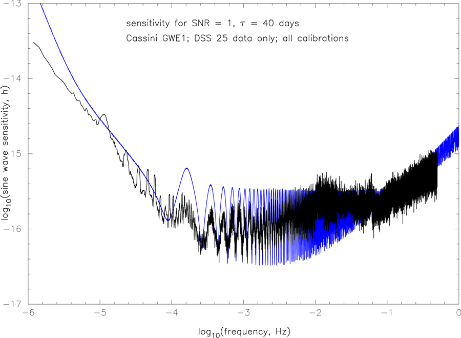
Sinusoidal sensitivity is traditionally stated as the amplitude h of a sinusoidal GW required to achieve a
specified SNR, as a function of Fourier frequency [18*, 113, 16*]. Conventionally, the signal is
averaged over the sky and over polarization state [52*, 127*, 16]. Figure 20* shows the all-sky
sensitivity based on a smoothed version of the actual spectrum (black curve) for the Cassini
2001 – 2002 observation. Cassini achieves  10–16 all-sky sensitivity over a fairly broad Fourier
band.
10–16 all-sky sensitivity over a fairly broad Fourier
band.
Early searches for periodic waves involved short duration observations (several hours to a few days; see,
e.g., [4, 18*]) and thus ignorable modulation of an astronomical sinusoid due to changing geometry
(non-time-shift-invariance of the GW transfer function; see Section 3). A true fixed-frequency signal would
be reflected in the spectrum of the (noisy) Doppler times series as a “Rice-squared” random
variable [97] at the signal frequency. Subsequent observations were over 10 – 40 days and the time
dependence of the earth-spacecraft-source geometry became important: A sinusoidal excitation
would be modulated into a non-sinusoidal Doppler response with power typically smeared over a
few Fourier frequency resolution bins. Non-negligible modulation has both advantages and
disadvantages. An advantage is that a real GW signal has a source-location-dependent signature in
the data and this can be used to verify or refute an astronomical origin of a candidate. The
disadvantage is that a simple spectral analysis is not sufficient for optimum detection (SNR
losses of the simple spectral analysis technique are frequency and geometry dependent but can
be  3 dB or more in some observations) and the computational cost to search for even a
simple astronomical-origin sinusoid becomes larger. Searches to date have addressed this with a
hierarchical approach to the data analysis. First a suboptimal-but-simple spectral analysis is
done. Candidates are then identified using an SNR threshold which is high enough to exclude
Fourier components which, even with proper analysis, would be too weak to be classified as
other-than-noise. The idea is to use a computationally inexpensive procedure (i.e., FFTs) to exclude
candidates which could not, in principle, be raised to a reasonable threshold SNR even with
accurate matched filtering. The frequencies of candidate signals passing the threshold are saved
and matched filters are constructed using the known time-dependence of the earth-spacecraft
geometry and for 20 points on the sky (the vertices of a dodecahedron projected onto the celestial
sphere.11)
3 dB or more in some observations) and the computational cost to search for even a
simple astronomical-origin sinusoid becomes larger. Searches to date have addressed this with a
hierarchical approach to the data analysis. First a suboptimal-but-simple spectral analysis is
done. Candidates are then identified using an SNR threshold which is high enough to exclude
Fourier components which, even with proper analysis, would be too weak to be classified as
other-than-noise. The idea is to use a computationally inexpensive procedure (i.e., FFTs) to exclude
candidates which could not, in principle, be raised to a reasonable threshold SNR even with
accurate matched filtering. The frequencies of candidate signals passing the threshold are saved
and matched filters are constructed using the known time-dependence of the earth-spacecraft
geometry and for 20 points on the sky (the vertices of a dodecahedron projected onto the celestial
sphere.11)
Linear chirp processing adds an additional parameter (chirp rate) and requires detection thresholds to be set higher. In both the sinusoidal and chirp analyses, the pdfs of signal power have been used to assess candidates (see, e.g., [18, 3, 32]). Non-linear chirps, if source parameters are favorable, could be strong candidate signals. Analysis methods, anticipated sensitivity, and detection range for Cassini are discussed in [30*].
6.3.2 Nonsinusoidal periodic waves
Calculations of Doppler response to GWs from a nonrelativistic binary system [127] show that the observed Doppler waveform can have a rich harmonic content. Monte Carlo calculations of GW strength from stars in highly elliptical orbits around the Galaxy’s central black hole have been given in [53]. For these stellar-mass secondaries generate wave amplitudes more than an order of magnitude weaker than Cassini-era Doppler sensitivity.
6.4 Burst waves
The first systematic search for burst radiation was done by filtering the data to de-emphasize
the dominant noise (plasma noise) relative to components of the time series anticorrelated
at the two-way light time [60]. Analysis of subsequent data sets used matched filtering with
assumed waveforms and targeted-sky-directions [7*, 63*, 64*]. The utility of multiple-spacecraft
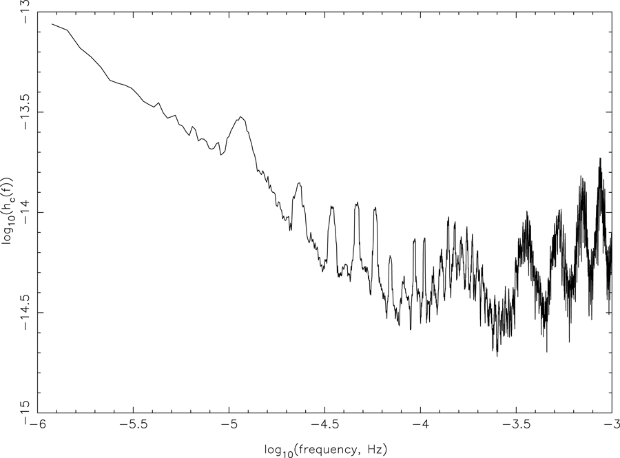
observations for burst searches was discussed by [28*, 112, 13]. Figure 21* is the crudest measure of
current-generation (Ka-band, tropospheric corrected) all-sky burst sensitivity. It shows the power
spectrum of two-way Doppler divided by the isotropic GW transfer function (see, e.g., [52*, 54*] and
Section 5.4) computed as [108] ![h (f) = [2fSgw ∕R¯ (f)]1∕2 c y2 2](article188x.gif) , where
, where  is the sky- and
polarization-averaged GW response function [52*, 54*, 19*]. The best sensitivity, hc < 2 ×10–15, occurs at
about 0.3 mHz, set by the minimization of the antenna mechanical noise through its transfer
function, the bandwidth, and the average coupling of the GW to the Doppler,
is the sky- and
polarization-averaged GW response function [52*, 54*, 19*]. The best sensitivity, hc < 2 ×10–15, occurs at
about 0.3 mHz, set by the minimization of the antenna mechanical noise through its transfer
function, the bandwidth, and the average coupling of the GW to the Doppler,  , at this
frequency.
, at this
frequency.
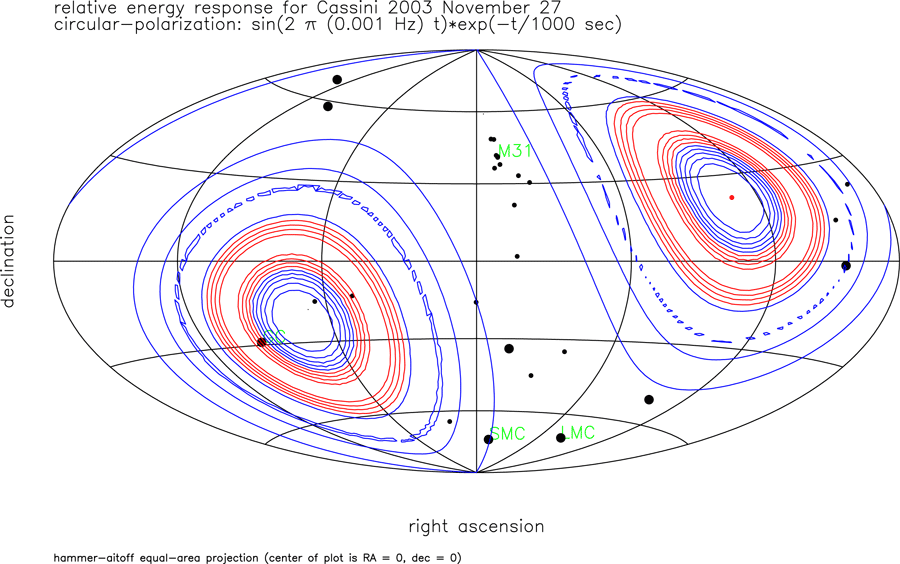
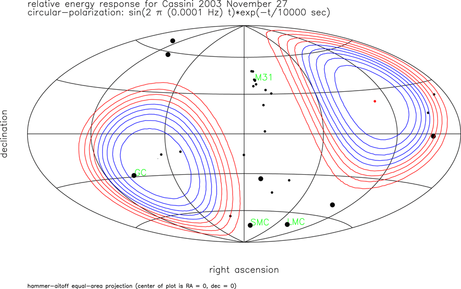
Sensitivity is not uniform over the sky and one can often do much better with knowledge of the direction-of-arrival or the waveform. Figure 22* shows contours of constant matched filter output for a circularly polarized mid-band burst wave using the Cassini solar opposition geometry of November 2003. The red dot shows the right ascension and declination of Cassini as viewed from the earth, the black dots are the positions of members of the Local Group of galaxies (larger dots indicating nearer objects), and “GC” marks the location of the galactic center. Contour levels are at 1/10 of the maximum, with red contours at 0.9 to 0.5 of the maximum filter output and blue contours at 0.4 to 0.1. The response is zero in the direction and anti-direction of the earth-Cassini vector (see Eq. (1*)). The angular response changes for GWs in the long-wavelength limit. Figure 23* similarly shows matched filter signal output contours, but for a burst wave with characteristic duration > T2. Pilot analyses using simplified waveforms [63, 11*] have been done accounting for the local non-stationarity of the noise and varying assumed source position on the sky.
 and
and  its Hilbert transform,
adapted from [64]. Cassini November 2003 geometry is assumed (the red dot is the right ascension
and declination of Cassini). Black dots are the positions of members of the Local Group of galaxies.
“GC” marks the location of the galactic center. Contour levels are at 1/10 of the maximum, with
red contours at 0.9 to 0.5 of the maximum signal output and blue contours at 0.4 to 0.1. Doppler
response is zero in the direction of Cassini (and its anti-direction).
its Hilbert transform,
adapted from [64]. Cassini November 2003 geometry is assumed (the red dot is the right ascension
and declination of Cassini). Black dots are the positions of members of the Local Group of galaxies.
“GC” marks the location of the galactic center. Contour levels are at 1/10 of the maximum, with
red contours at 0.9 to 0.5 of the maximum signal output and blue contours at 0.4 to 0.1. Doppler
response is zero in the direction of Cassini (and its anti-direction). Waves from coalescing binary sources are intermediate between periodic and burst waves. Expected
sensitivity and analysis methods have been treated in detail by Bertotti, Iess, and Vecchio [30*, 124];
supermassive black hole coalescences with favorable parameters are visible with Cassini-class sensitivity out
to 100s of Mpc. Cassini is also sensitive to  intermediate-mass black holes coalescing with the
supermassive black hole at the galactic center [30].
intermediate-mass black holes coalescing with the
supermassive black hole at the galactic center [30].
 and
and  its Hilbert transform. This model waveform is long compared with
 6.5 Sensitivity to a stochastic background
A stochastic background of low-frequency GWs, potentially detectable with single or multiple spacecraft
Doppler tracking, has been discussed by [52, 26, 58, 82, 6, 28, 44, 7, 54, 19*]. The level of stochastic
GWs is conventionally expressed either as the energy density in GWs relative to closure density,  , as a
characteristic rms strain, or as spectrum of strain. The best directly observational upper bounds on
stochastic GWs in the low-frequency band come from the Cassini data. Details of how the upper
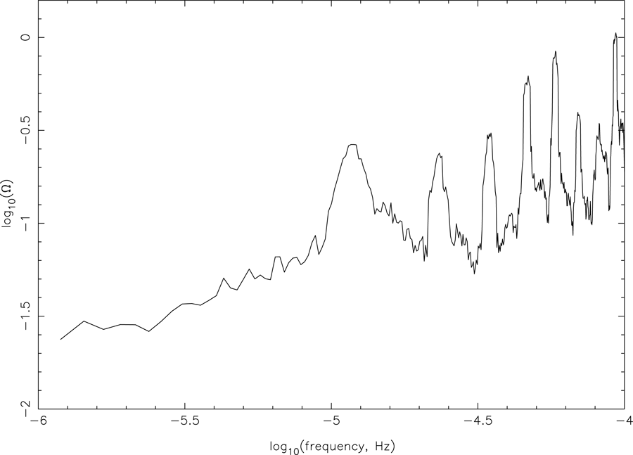
limits were produced are given in [19*]. Figure 24* shows limits to
, as a
characteristic rms strain, or as spectrum of strain. The best directly observational upper bounds on
stochastic GWs in the low-frequency band come from the Cassini data. Details of how the upper
limits were produced are given in [19*]. Figure 24* shows limits to  as a function of Fourier
frequency (upper limits expressed as spectrum of strain are given in [19*]). The lowest bound is at
1.2 × 10⁻⁶ Hz :
as a function of Fourier
frequency (upper limits expressed as spectrum of strain are given in [19*]). The lowest bound is at
1.2 × 10⁻⁶ Hz :  < 0.025. Between 1.2 × 10⁻⁶ and
  10–5 Hz,
  < 0.1, while between about
10–5 – 10–4 Hz the upper bounds are between 0.1 to about 1.0. For f > 10–4 Hz the limits
to
< 0.1, while between about
10–5 – 10–4 Hz the upper bounds are between 0.1 to about 1.0. For f > 10–4 Hz the limits
to  are larger than 1. The Cassini data improved limits to
  in the 10–6 to 10–4 Hz
band by factors of 500 – 1200 (depending on Fourier frequency) compared with earlier Doppler
experiments.
in the 10–6 to 10–4 Hz
band by factors of 500 – 1200 (depending on Fourier frequency) compared with earlier Doppler
experiments.
Predictions for an astrophysical GW background in the low-frequency band, e.g., from an ensemble of galactic binary stars or an ensemble of massive black hole binaries, have mainly been aimed at the design sensitivity of future dedicated GW missions [24*]. The galactic binary star background is much too weak to be seen with spacecraft Doppler tracking. At lower frequencies (10–9 – 10–6 Hz) the strength of a GW background from an ensemble of coalescing black hole binaries has been estimated [93, 72*, 132*] mostly in the context of a pulsar timing array. Extrapolations or predictions in the low-frequency band [72, 132] give strengths substantially lower than spacecraft Doppler tracking can presently observe (see Figure 21*).
 |
 |
 |