2 The Theory of Gravitation
Newton’s theory of gravitation provided a description of the effect of gravity through the inverse square law without attempting to explain the origin of gravity. The inverse square law provided an accurate description of all measured phenomena in the solar system for more than two hundred years, but the first hints that it was not the correct description of gravitation began to appear in the late 19th century, as a result of the improved precision in measuring phenomena such as the perihelion precession of Mercury. Einstein’s contribution to our understanding of gravity was not only practical but also aesthetic, providing a beautiful explanation of gravity as the curvature of spacetime. In developing GR as a generally covariant theory based on a dynamical spacetime metric, Einstein sought to extend the principle of relativity to gravitating systems, and he built on the crucial 1907 insight that the equality of inertial and gravitational mass allowed the identification of inertial systems in homogeneous gravitational fields with uniformly accelerated frames – the principle of equivalence [339]. Einstein was also guided by his appreciation of Ricci and Levi-Civita’s absolute differential calculus (later to become differential geometry), arguably as much as by the requirement to reproduce Newtonian gravity in the weak-field limit. Indeed, one could say that GR was born “of almost pure thought” [471 ].
].
Einstein’s theory of GR is described by the action
in which
 is the determinant of the spacetime metric and
  is the Ricci scalar,
where
is the Ricci scalar,
where  is the Ricci Tensor,
  the Riemann
curvature tensor,
the Riemann
curvature tensor,  the affine connection, and a comma denotes a
partial derivative. When coupled to a matter distribution, this action yields the field equations
where
the affine connection, and a comma denotes a
partial derivative. When coupled to a matter distribution, this action yields the field equations
where 
 denotes the stress-energy tensor of the matter.
Since the development of the theory, GR has withstood countless experimental tests [471, 443, 444]
based on measurements as different as atomic-clock precision [378], orbital dynamics (most notably lunar
laser ranging [309]), astrometry [415], and relativistic astrophysics (most exquisitely the binary pulsar
[293, 471], but not only [372]). It is therefore the correct and natural benchmark against which to compare
alternative theories using future observations and we will follow the same approach in this
article. Unlike in the case of Newtonian gravity at the time that GR was developed, there are
no current observations that GR cannot explain that can be used to guide development of
alternatives.1
Nonetheless, there are crucial aspects of Einstein’s theory that have never been probed directly, such as its
strong-field dynamics and the propagation of field perturbations (GWs). Furthermore, it is known that
classical GR must ultimately fail at the Planck scale, where quantum effects become important, and traces
of the quantum nature of gravity may be accessible at lower energies [400]. As emphasized by Will [471],
GR has no adjustable constants, so every test is potentially deadly, and a probe that could reveal new
physics.
2.1 Will’s “standard model” of gravitational theories
Will’s Living Review [471] and his older monograph [469] are the fundamental references about the
experimental verification of GR. In this section, we give only a brief overview of what may be called Will’s
“standard model” for alternative theories of gravity, which proceeds through four steps: a) strong evidence
for the equivalence principle supports a metric formulation for gravity; b) metric theories are classified
according to what gravitational fields (scalar, vector, tensor) they prescribe; c) slow-motion, weak-field
conservative dynamics are described in a unified parameterized post-Newtonian (PPN) formalism, and
constrained by experiment and observations; d) finally, equations for the slow-motion generation and
weak-field propagation of gravitational radiation are derived separately for each metric theory, and again
compared to observations. Many of the tests of gravitational physics envisaged for LISA belong
in this last sector of Will’s standard model, and are discussed in Section 5.1 of this review.
This scheme however leaves out two other important points of contact between gravitational
phenomenology and LISA’s GW observations: the strong-field, nonlinear dynamics of black
holes and their structure and excitations, especially as probed by small orbiting bodies. We will
deal with these in Sections 5 and 6, respectively; but let us first delve into Will’s standard
model.
The equivalence principle and metric theories of gravitation.
Einstein’s original intuition [338] placed the equivalence principle [222] as a cornerstone for the theories that describe gravity as curved spacetime. As formulated by Newton, the principle states simply that inertial and gravitational mass are proportional, and therefore all “test” bodies fall with the same acceleration (in modern usage, this is known as the weak equivalence principle, or WEP). Dicke later recognized that in developing GR Einstein had implicitly posited a broader principle (Einstein’s equivalence principle, or EEP) that consists of WEP plus local Lorentz invariance and local position invariance: that is, of the postulates that the outcome of local non-gravitational experiments is independent of, respectively, the velocity and position of the local freely-falling reference frames in which the experiments are performed.|
|
|
|
|
Turyshev [443] gives a current review of the experimental verification of WEP (shown to
hold to parts in 1013 by differential free-fall tests [399]), local Lorentz invariance (verified to
parts in 1022 by clock-anisotropy experiments [276]), and local position invariance (verified to
parts in 105 by gravitational-redshift experiments [58], and to much greater precision when
looking for possible time variations of fundamental constants [445]). Although these three parts of
EEP appear distinct in their experimental consequences, their underlying physics is necessarily
related in any theory of gravity, so Schiff conjectured (and others argued convincingly) that
any complete and self-consistent theory of gravity that embodies WEP must also realize EEP
[471].
EEP leads to metric theories of gravity in which spacetime is represented as a pseudo-Riemannian
manifold, freely-falling test bodies move along the geodesics of its metric, and non-gravitational physics is
obtained by applying special-relativistic laws in local freely-falling frames. GR is, of course,
a metric theory of gravity; so are scalar-vector-tensor theories such as Brans–Dicke theory,
which include other gravitational fields in addition to the metric. By contrast, theories with
dynamically varying fundamental constants and theories (such as superstring theory) that introduce
additional WEP-violating gravitational fields [471, Section 2.3] are not metric. Neither are
most theories that provide short-range and long-range modifications to Newton’s inverse-square
law [3].
The scalar and vector fields in scalar-vector-tensor theories cannot directly affect the motion of matter and other non-gravitational fields (which would violate WEP), but they can intervene in the generation of gravity and modify its dynamics. These extra fields can be dynamical (i.e., determined only in the context of solving for the evolution of everything else) or absolute (i.e., assigned a priori to fixed values). The Minkowski metric of special relativity is the classic example of absolute field; such fields may be regarded as philosophically unpleasant by those who dislike feigning hypotheses, but they have a right of citizenship in modern physics as “frozen in” solutions from higher energy scales or from earlier cosmological evolution.
The additional fields can potentially alter the outcome of local gravitational experiments: while the local gravitational effects of different metrics far away can always be erased by describing physics in a freely-falling reference frame (which is to say, the local boundary conditions for the metric can be arranged to be flat spacetime), the same is not true for scalar and vector fields, which can then affect local gravitational dynamics by their interaction with the metric. This amounts to a violation not of EEP, but of the strong equivalence principle (SEP), which states that EEP is also valid for self-gravitating bodies and gravitational experiments. SEP is verified to parts in 104 by combined lunar laser-ranging and laboratory experiments [476]. So far, GR appears to be the only viable metric theory that fully realizes SEP.
The PPN formalism.
Because the experimental consequences of different metric theories follow from the specific metric that is generated by matter (possibly with the help of the extra gravitational fields), and because all these theories must realize Newtonian dynamics in appropriate limiting conditions, it is possible to parameterize them in terms of the coefficients of a slow-motion, weak-field expansion of the metric. These coefficients appear in front of gravitational potentials similar to the Newtonian potential, but involving also matter velocity, internal energy, and pressure. This scheme is the parameterized post-Newtonian formalism, pioneered by Nordtvedt and extended by Will (see [469] for
details).
Of the ten PPN parameters in the current version of the formalism, two are the celebrated  and
and  (already introduced by Eddington, Robertson, and Schiff for the “classical” tests of GR) that rule,
respectively, the amount of space curvature produced by unit rest mass and the nonlinearity in the
superposition of gravitational fields. In GR,
(already introduced by Eddington, Robertson, and Schiff for the “classical” tests of GR) that rule,
respectively, the amount of space curvature produced by unit rest mass and the nonlinearity in the
superposition of gravitational fields. In GR,  and
and  each have the value 1. The other eight parameters,
if not zero, give origin to violations of position invariance (
each have the value 1. The other eight parameters,
if not zero, give origin to violations of position invariance ( ), Lorentz invariance (
 ), or even of
the conservation of total momentum (
), or even of
the conservation of total momentum ( ,
,  ) and total angular momentum (
 ,
,
 ).
).
The PPN formalism is sufficiently accurate to describe the tests of gravitation performed
in the solar system, as well as many tests using binary-pulsar observations. The parameter
 is currently constrained to 1 ± a few 10–5 by tests of light delay around massive
bodies using the Cassini spacecraft [81];
is currently constrained to 1 ± a few 10–5 by tests of light delay around massive
bodies using the Cassini spacecraft [81];  to 1 ± a few 10–4 by lunar laser ranging
[476].2
The other PPN parameters have comparable bounds around zero from solar-system and pulsar
measurements, except for
to 1 ± a few 10–4 by lunar laser ranging
[476].2
The other PPN parameters have comparable bounds around zero from solar-system and pulsar
measurements, except for  , which is known exceedingly well from pulsar observations [471].
2.2 Alternative theories
Tests in the PPN framework have tightly constrained the field of viable alternatives to GR, largely
excluding theories with absolute elements that give rise to preferred-frame effects [471]. The
(indirect) observation of GW emission from the binary pulsar and the accurate prediction of its
 by Einstein’s quadrupole formula have definitively excluded other theories [471, 422]. Yet
more GR alternatives were conceived to illuminate points of principle, but they are not well
motivated physically and therefore are hardly candidates for experimental verification. Some of
the theories that are still “alive” are described in the following. More details can be found
in [469].
by Einstein’s quadrupole formula have definitively excluded other theories [471, 422]. Yet
more GR alternatives were conceived to illuminate points of principle, but they are not well
motivated physically and therefore are hardly candidates for experimental verification. Some of
the theories that are still “alive” are described in the following. More details can be found
in [469].
2.2.1 Scalar-tensor theories
The addition of a single scalar field  to GR produces a theory described by the Einstein-frame action
(see, e.g., [471]),
to GR produces a theory described by the Einstein-frame action
(see, e.g., [471]),
 d x + Imatter(ψm, A (φ)&tidle;gμν), (3 )](article26x.gif)
 is the metric, the Ricci curvature scalar
  yields the general-relativistic Einstein–Hilbert
action, and the two adjacent terms are kinetic and potential energies for the scalar field. Note that in the
action
yields the general-relativistic Einstein–Hilbert
action, and the two adjacent terms are kinetic and potential energies for the scalar field. Note that in the
action  for matter dynamics, the metric couples to matter through the function
  , so this
representation is not manifestly metric; it can however be made so by a change of variables that yields the
Jordan-frame action,
where
, so this
representation is not manifestly metric; it can however be made so by a change of variables that yields the
Jordan-frame action,
where  d x + Imatter(ψm, gμν), (4 )](article31x.gif)
 is the transformed scalar field,
 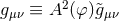 is the physical metric underlying
gravitational observations, and
is the physical metric underlying
gravitational observations, and ![3 + 2ω (ϕ) ≡ [d (ln A(φ ))∕d φ]−2](article34x.gif) .
.
The “classic” Brans–Dicke theory corresponds to fixing  to a constant
  , and it is
indistinguishable from GR in the limit
, and it is
indistinguishable from GR in the limit  . In the PPN framework, the only parameter that differs
from GR is
. In the PPN framework, the only parameter that differs
from GR is  . Damour and Esposito-Farèse [142] considered an expansion of
 around a cosmological background value,

 (and further coefficients)
  reproduces Brans–Dicke with
  ,
,  causes the evolution of the scalar field toward
  (and therefore toward GR); and
  may allow a
phase change inside objects like neutron stars, leading to large SEP violations. These parameters are bound
by solar-system, binary-pulsar, and GW observations [143, 186].
may allow a
phase change inside objects like neutron stars, leading to large SEP violations. These parameters are bound
by solar-system, binary-pulsar, and GW observations [143, 186].
Scalar-tensor theories have found motivation in string theory and cosmological models, and have attracted the most attention in terms of tests with GW observations.
2.2.2 Vector-tensor theories
These are obtained by including a dynamical vector field  coupled to the metric tensor. The most
general second-order action in such a theory takes the form [471]
coupled to the metric tensor. The most
general second-order action in such a theory takes the form [471]
![∫ 1 4 √ --- [ ν μν α β μ ] S = ------ d x − g (1 + ωu μu )R − K αβu;μu;ν + λ(u μu + 1) , μν 16πGμν μ ν μ ν μ ν where K αβ = c1g gαβ + c2δαδβ + c3δβ δα − c4u u gαβ , (6 )](article48x.gif)
 are arbitrary constants.
There are two types of vector-tensor theories: in unconstrained theories,
are arbitrary constants.
There are two types of vector-tensor theories: in unconstrained theories,  and the constant
  is
arbitrary, while in Einstein-aether theories the vector field
is
arbitrary, while in Einstein-aether theories the vector field  is constrained to have unit norm, so the
Lagrange multiplier
is constrained to have unit norm, so the
Lagrange multiplier  is arbitrary and the constraint allows
  to be absorbed into a rescaling of
  .
For the unconstrained theory, only versions of the theory with
.
For the unconstrained theory, only versions of the theory with  have been studied and for these the
field equations are [469]
where
have been studied and for these the
field equations are [469]
where ![1 R κλ − -Rg κλ + ωΘ (κωλ)+ η Θ(κηλ)+ 𝜖Θ (𝜖κ)λ + τΘ (τκ)λ + Λgκλ = 0 , 2 𝜖F ;ν + 1τu;ν − 1ωu R − 1ηu αR = 0, μν 2 μ;ν 2 μ 2 μα (ω ) 2 1- 2 2 2 Θ κλ = u κuλR + u Rκλ − 2 gκλu R − (u );κλ + gκλ□gu , 1 1 1 Θ (κηλ)= 2u αu[κRλ]α − -gκλu αuβR αβ − (u αu[κ);λ]α + --□g (u κuλ) + -gκλ(uαu β);αβ , 2 2 2 Θ(𝜖)= − 2(F αF − 1g F Fαβ) , κλ κ λα 4 κλ αβ (τ) ;α α 1- α;β α α ;α Θ κλ = uκ;αuλ + u α;κu;λ − 2gκλu α;βu + (u u[κ;λ] − u;[κuλ] − u [κuλ]);α , (7 )](article57x.gif)
 ,
,  ,
,  ,
,  , and
, and  . We use
the usual subscript notation, such that “
. We use
the usual subscript notation, such that “ ” and “
![[,]](article64x.gif) ” denote symmetric and antisymmetric
sums.
” denote symmetric and antisymmetric
sums.
In the constrained Einstein-aether theory [250] the field equations are
where![α α α J μ;α − c4u˙ u;μ = λuμ , where Jα ≡ K αβuν , μ μν ;β (u) 8πG-- matter G αβ = Tαβ + c4 Tαβ , (u) ( μ μ μ) ( α ;μ μ) Tαβ ≡ J(α uβ) − J (αuβ) − J(α β)u ;μ + c1 u;μuβ − uμ;αu ;β + c4˙uαu˙β [ μν 2] 1 + uνJ;μ − c4˙u u αuβ − 2g αβLu , (8 )](article65x.gif)
 ,
,  is the aether Lagrangian, and
  is the usual matter
stress-energy tensor [163]. Via field redefinition this theory can be shown to be equivalent to GR if
is the usual matter
stress-energy tensor [163]. Via field redefinition this theory can be shown to be equivalent to GR if
 ,
,  , and
, and  [57]. Field redefinition can also be used to set
 [185]; if this constraint is imposed then equivalence to GR is only achieved if the
  are all
zero. This constraint is therefore appropriate to pose Einstein-aether theory as an alternative to test
against GR, since then any non-zero values of the
are all
zero. This constraint is therefore appropriate to pose Einstein-aether theory as an alternative to test
against GR, since then any non-zero values of the  would represent genuine deviations from
GR.
would represent genuine deviations from
GR.
Unconstrained vector-tensor theories were introduced in the 1970s as a straw-man alternative to
GR [469], but they have four arbitrary parameters and leave the magnitude of the vector field
unconstrained, which is a serious defect. Interest in Einstein-aether theories was prompted by
the desire to construct a covariant theory that violated Lorentz invariance under boosts, by
having a preferred reference frame – the aether, represented by the vector  . The preferred
reference frame also provides a universal notion of time [202]. Interest in theories that violate
Lorentz symmetry has recently been revived as a possible window onto aspects of quantum
gravity [22].
. The preferred
reference frame also provides a universal notion of time [202]. Interest in theories that violate
Lorentz symmetry has recently been revived as a possible window onto aspects of quantum
gravity [22].
2.2.3 Scalar-vector-tensor theories
The natural extension of scalar-tensor and vector-tensor theories are scalar-vector-tensor theories in which the gravitational field is coupled to a vector field and one or more scalar fields. These theories are relativistic generalizations of Modified Newtonian Dynamics (MoND), which was proposed in order to reproduce observed rotation curves on galactic scales. The relativistic extensions were designed to also satisfy cosmological observations on larger scales. The action takes the form
where
 and
and  are the usual gravitational and matter Lagrangians. There are two
main versions of the theory, which differ in the choice of the scalar-field and vector-field Lagrangians
are the usual gravitational and matter Lagrangians. There are two
main versions of the theory, which differ in the choice of the scalar-field and vector-field Lagrangians  and
and  .
.
In Tensor-Vector-Scalar gravity (TeVeS) [61] the dynamical vector field  is coupled to a dynamical
scalar field
is coupled to a dynamical
scalar field  . A second scalar field
  is here considered non-dynamical. The Lagrangians are
![1 [ ( ) 1 G ] LS = --- σ2 gα β − u αuβ ϕ,αϕ,β + ---2σ4F (G σ2) , 2G [ 2 l ] K-- αβ μν λ-- μ Lu = 2G g g B αμB βν + 2 K (u uμ + 1) , (10 )](article84x.gif)
 ,
,  is an unspecified dimensionless function,
  is a dimensionless parameter,
and
is a dimensionless parameter,
and  is a constant length parameter. The Lagrange multiplier
  is spacetime dependent, set to enforce
normalization of the vector field
is spacetime dependent, set to enforce
normalization of the vector field  . In TeVeS the physical metric that governs the gravitational
dynamics of ordinary matter does not coincide with
. In TeVeS the physical metric that governs the gravitational
dynamics of ordinary matter does not coincide with  , but is determined by the scalar field through
An alternative version of TeVeS, called Bi-Scalar-Tensor-Vector gravity (BSTV) has also been
proposed [392], in which the scalar field
, but is determined by the scalar field through
An alternative version of TeVeS, called Bi-Scalar-Tensor-Vector gravity (BSTV) has also been
proposed [392], in which the scalar field 
 is allowed to be dynamical. TeVeS is able to explain galaxy
rotation curves and satisfies constraints from cosmology and gravitational lensing, but stars are very
unstable [402] and the Bullet cluster [123] observations (which point to dark matter) cannot be
explained.
is allowed to be dynamical. TeVeS is able to explain galaxy
rotation curves and satisfies constraints from cosmology and gravitational lensing, but stars are very
unstable [402] and the Bullet cluster [123] observations (which point to dark matter) cannot be
explained.
In Scalar-Tensor-Vector Gravity (STVG) [317] the Lagrangian for the vector field is taken to be
with![[ μν 2 μ ] Lu = ω B Bμν − 2μ u uμ + Vu(u) , (12 )](article94x.gif)
 defined as before. The three constants
  ,
,  , and G that enter this action and the
gravitational action are then taken to be scalar fields governed by the Lagrangian
It is claimed that STVG predicts no deviations from GR on the scale of the solar system or for small
globular clusters [319], and that it can reproduce galactic rotation curves [97], gravitational lensing in the
Bullet cluster [98], and a range of cosmological observations [318]. TeVeS-like theories are constrained by
binary-pulsar observations [186]. It has been proposed that an extension of the ESA-led LISA
Pathfinder technology-demonstration mission may allow additional constraints on this class of
theories [301]. To date the consequences of TeVeS or STVG for GW observations have not been
investigated.
, and G that enter this action and the
gravitational action are then taken to be scalar fields governed by the Lagrangian
It is claimed that STVG predicts no deviations from GR on the scale of the solar system or for small
globular clusters [319], and that it can reproduce galactic rotation curves [97], gravitational lensing in the
Bullet cluster [98], and a range of cosmological observations [318]. TeVeS-like theories are constrained by
binary-pulsar observations [186]. It has been proposed that an extension of the ESA-led LISA
Pathfinder technology-demonstration mission may allow additional constraints on this class of
theories [301]. To date the consequences of TeVeS or STVG for GW observations have not been
investigated.
![[ ( ) ] LS = 16π- 1-gνρ G,νG,ρ-+ μ,νμ,ρ-− ω,νω,ρ + VG-(G-)+ Vμ(μ)-+ V ω(ω) . (13 ) G 2 G2 μ2 G2 μ2](article98x.gif)
2.2.4 Modified-action theories
f(R) gravity.
This theory is derived by replacing with an arbitrary function
  in the
Einstein–Hilbert action. There are two versions of
in the
Einstein–Hilbert action. There are two versions of  gravity. In the metric formalism the action is
extremized with respect to the metric coefficients only, and the connection is taken to be the metric
connection, depending on the metric components in the standard way. The resulting field equations are
In the Palatini formalism, the field equations are found by extremizing the action over both the metric and
the connection. For an
gravity. In the metric formalism the action is
extremized with respect to the metric coefficients only, and the connection is taken to be the metric
connection, depending on the metric components in the standard way. The resulting field equations are
In the Palatini formalism, the field equations are found by extremizing the action over both the metric and
the connection. For an 
 action the resulting equations are
If the second derivative
action the resulting equations are
If the second derivative ![′ 1- [√ --- ′ κλ] Rκλf (R ) − 2gκλf(R ) = 0, ∇ α − gf (R)g = 0 . (15 )](article104x.gif)
 , metric
  gravity can be shown to be equivalent to a Brans–Dicke
theory with
gravity can be shown to be equivalent to a Brans–Dicke
theory with  , while Palatini
  gravity is equivalent to a Brans–Dicke theory with
 , with no constraint imposed on
  [180, 419, 146]. In both cases, the Brans–Dicke
potential depends on the exact functional form
[180, 419, 146]. In both cases, the Brans–Dicke
potential depends on the exact functional form  .
.
 theories have attracted a lot of interest in a cosmological context, since the flexibility in choosing
the function
theories have attracted a lot of interest in a cosmological context, since the flexibility in choosing
the function  allows a wide range of cosmological phenomena to be described [336, 108], including
inflation [423, 459] and late-time acceleration [107, 112], without violating constraints from
Big-Bang Nucleosynthesis [168]. However, metric
allows a wide range of cosmological phenomena to be described [336, 108], including
inflation [423, 459] and late-time acceleration [107, 112], without violating constraints from
Big-Bang Nucleosynthesis [168]. However, metric  theories are strongly constrained by
solar-system and laboratory measurements if the scalar degree of freedom is assumed to be
long-ranged, which modifies the form of the gravitational potential [121]. This problem can be avoided
by assuming a short-range scalar field, but then
theories are strongly constrained by
solar-system and laboratory measurements if the scalar degree of freedom is assumed to be
long-ranged, which modifies the form of the gravitational potential [121]. This problem can be avoided
by assuming a short-range scalar field, but then  theories can only explain the early
expansion of the universe and not late-time acceleration. The Chameleon mechanism [262] has been
invoked to circumvent this, as it allows the scalar-field mass to be a function of curvature, so
that the field can be short ranged within the solar system but long ranged on cosmological
scales.
theories can only explain the early
expansion of the universe and not late-time acceleration. The Chameleon mechanism [262] has been
invoked to circumvent this, as it allows the scalar-field mass to be a function of curvature, so
that the field can be short ranged within the solar system but long ranged on cosmological
scales.
There are also other issues with  theories. For example, in Palatini
  gravity the
post-Newtonian metric depends on the local matter density [418], while in metric
gravity the
post-Newtonian metric depends on the local matter density [418], while in metric  gravity with
 there is a Ricci-scalar instability [153] that arises because the effective gravitational constant
increases with increasing curvature, leading to a runaway instability for small stars [56, 55]. We refer
the reader to [419, 146] for more complete reviews of the current understanding of
there is a Ricci-scalar instability [153] that arises because the effective gravitational constant
increases with increasing curvature, leading to a runaway instability for small stars [56, 55]. We refer
the reader to [419, 146] for more complete reviews of the current understanding of  gravity.
Chern–Simons gravity.
Yunes and others [6, 8, 12, 13, 103, 104, 111, 158, 189, 212, 218, 272, 323, 416, 488, 491, 496, 501, 503, 499, 340]
have recently developed an extensive analysis of the observational consequences of Jackiw and Pi’s
Chern–Simons gravity [249], which extends the Hilbert action with an additional Pontryagin term  that is quadratic in the Riemann tensor [212]:
here
that is quadratic in the Riemann tensor [212]:
here  d x + Imatter(ψm, gμν); (16 )](article122x.gif)
 is built with the help of the dual Riemann tensor
  ,
and it can be expressed as the divergence of the gravitational Chern–Simons topological
current;3
the scalar field
,
and it can be expressed as the divergence of the gravitational Chern–Simons topological
current;3
the scalar field  can be treated either as a dynamical quantity, or an absolute field. In both
cases,
can be treated either as a dynamical quantity, or an absolute field. In both
cases,  vanishes, either dynamically, or as a constraint on acceptable solutions, needed to
enforce coordinate-invariant matter dynamics, which restricts the space of solutions available to
GR.
Chern–Simons gravity is motivated by string theory and by the attempt to develop a quantum theory of
gravity satisfying a gauge principle. The Pontryagin term arises in the standard model of particle physics as
a gauge anomaly: the classical gravitational Noether current that comes from the symmetry of the
gravitational action is no longer conserved when the theory is quantized, but has a divergence proportional
to the Pontryagin term. This anomaly can be canceled by modifying the action via the addition of the
Chern–Simons Pontryagin term. The same type of correction arises naturally in string theory through the
Green–Schwarz anomaly-canceling mechanism, and in Loop Quantum Gravity to enforce parity and
charge-parity conservation.
vanishes, either dynamically, or as a constraint on acceptable solutions, needed to
enforce coordinate-invariant matter dynamics, which restricts the space of solutions available to
GR.
Chern–Simons gravity is motivated by string theory and by the attempt to develop a quantum theory of
gravity satisfying a gauge principle. The Pontryagin term arises in the standard model of particle physics as
a gauge anomaly: the classical gravitational Noether current that comes from the symmetry of the
gravitational action is no longer conserved when the theory is quantized, but has a divergence proportional
to the Pontryagin term. This anomaly can be canceled by modifying the action via the addition of the
Chern–Simons Pontryagin term. The same type of correction arises naturally in string theory through the
Green–Schwarz anomaly-canceling mechanism, and in Loop Quantum Gravity to enforce parity and
charge-parity conservation.
The presence of the Chern–Simons correction leads to parity violation, which has various observable consequences, with magnitude depending on the Chern–Simons coupling, which string theory predicts will be at the Planck scale. If so, these effects will never be observable, but various mechanisms have been proposed that could enhance the strength of the Chern–Simons coupling, such as non-perturbative instanton corrections [433], fermion interactions [10], large intrinsic curvatures [9] or small string couplings at late times [468]. For further details on all aspects of Chern–Simons gravity, we refer the reader to [11].
General quadratic gravity.
This theory arises by adding to the action all possible terms that are quadratic in the Ricci scalar, Ricci tensor, and Riemann tensor. For the action the field equations are [372 ]
This class of theories is parameterized by the coefficients
]
This class of theories is parameterized by the coefficients 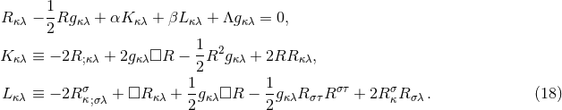
 ,
,  , and
, and  . More recently, Stein and
Yunes [504] considered a more general form of quadratic gravity that includes the Pontryagin term from
Chern–Simons gravity. Their action was
in which the
. More recently, Stein and
Yunes [504] considered a more general form of quadratic gravity that includes the Pontryagin term from
Chern–Simons gravity. Their action was
in which the ![∫ { √ --- 2 ab abcd S ≡ − g κR + α1f1 (𝜃)R + α2f2(𝜃)RabR + α3f3(𝜃)RabcdR } ∗ abcd β- a + α4f4(𝜃)R abcdR − 2 [∇a 𝜃∇ 𝜃 + 2V (𝜃)] + ℒmatter , (19 )](article132x.gif)
 and
and  are coupling constants,
  is a scalar field, and
  is the
matter Lagrangian density as before. There are two versions of this theory: a non-dynamical
version in which the functions
is the
matter Lagrangian density as before. There are two versions of this theory: a non-dynamical
version in which the functions  are constants, and a dynamical version in which they are
not.
General quadratic theories are known to exhibit ghost fields – negative mass-norm states that violate
unitarity (see, e.g., [419] for a discussion and further references). These occur generically, although models
with an action that is a function only of
are constants, and a dynamical version in which they are
not.
General quadratic theories are known to exhibit ghost fields – negative mass-norm states that violate
unitarity (see, e.g., [419] for a discussion and further references). These occur generically, although models
with an action that is a function only of  and
and  only are ghost-free [126].
Ghost fields are also present in Chern–Simons modified gravity [323, 158], which places strong constraints
on the parameters of that model.
only are ghost-free [126].
Ghost fields are also present in Chern–Simons modified gravity [323, 158], which places strong constraints
on the parameters of that model.
2.2.5 Massive-graviton theories
Massive-graviton theories were first considered by Pauli and Fierz [350, 175, 176], whose theory is
generated by an action of the form
![∫ [ S = M 2 d4x − 1(∂ h )2 + 1(∂ h)2 − 1(∂ )(∂νhμ ) + 1-(∂ h )(∂νhμρ) PF P 4 μ νρ 4 μ 2 μ ν 2 μ νρ ( ) ] − 1-m2 hμνhμν − h2 + M P−2Tμνhμν , (20 ) 4](article140x.gif)
 is a rank-two covariant tensor,
  and
and  are mass parameters,
  is the matter
energy-momentum tensor, indices are raised and lowered with the Minkowski metric
is the matter
energy-momentum tensor, indices are raised and lowered with the Minkowski metric  , and
, and
 . The terms on the first line of this expression are generated by expanding the Einstein–Hilbert
action to quadratic order in
. The terms on the first line of this expression are generated by expanding the Einstein–Hilbert
action to quadratic order in  . The massive graviton term is
 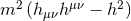 ; it contains a spin-2
piece
; it contains a spin-2
piece  and a spin-0 piece
  .
.
This model suffers from the van Dam–Velten–Zakharov discontinuity [454, 505]: no matter how small the graviton mass, the Pauli–Fierz theory leads to different physical predictions from those of linearized GR, such as light bending. The theory also predicts that the energy lost into GWs from a binary is twice the GR prediction, which is ruled out by current binary-pulsar observations. It might be possible to circumvent these problems and recover GR in the weak-field limit by invoking the Vainshtein mechanism [446, 41], which relies on nonlinear effects to “hide” certain degrees of freedom for source distances smaller than the Vainshtein radius [40]. The massive graviton can therefore become effectively massless, recovering GR on the scale of the solar system and in binary-pulsar tests, while retaining a mass on larger scales. In such a scenario, the observational consequences for GWs would be a modification to the propagation time for cosmological sources, but no difference in the emission process itself.
There are also non-Pauli–Fierz massive graviton theories [36]. For these, the action is the same as that
in Eq. (20 ), but the first term on the second line (the massive graviton term) takes the more general form

 and
and  are new constants of the theory that represent the squared masses of the spin-2 and
spin-0 gravitons respectively. This theory can recover GR in the weak field, since
are new constants of the theory that represent the squared masses of the spin-2 and
spin-0 gravitons respectively. This theory can recover GR in the weak field, since  and
and
 can independently be taken to zero, with modifications to weak-field effects that are on
the order of the graviton mass squared. These theories are generally thought to suffer from
instabilities [350, 175, 176], which arise because the spin-0 graviton carries negative energy. However, it
was shown in [36] that the spin-0 graviton cannot be emitted without spin-2 gravitons also being generated.
The spin-2 graviton energy is positive and greater than that of spin-2 gravitons in GR, which
compensates for the spin-0 graviton’s negative energy. The total energy emitted is therefore always
positive, and it converges to the GR value in the limit that the spin-2 graviton mass goes to
zero.
can independently be taken to zero, with modifications to weak-field effects that are on
the order of the graviton mass squared. These theories are generally thought to suffer from
instabilities [350, 175, 176], which arise because the spin-0 graviton carries negative energy. However, it
was shown in [36] that the spin-0 graviton cannot be emitted without spin-2 gravitons also being generated.
The spin-2 graviton energy is positive and greater than that of spin-2 gravitons in GR, which
compensates for the spin-0 graviton’s negative energy. The total energy emitted is therefore always
positive, and it converges to the GR value in the limit that the spin-2 graviton mass goes to
zero.
These alternative massive-graviton theories are therefore perfectly compatible with current observational constraints, but make very different predictions for strong gravitational fields [36], including the absence of horizons for black-hole spacetimes and oscillatory cosmological solutions. Despite these potential problems, the existence of a “massive graviton” can be used as a convenient strawman for GW constraints, since the speed of GW propagation can be readily inferred from GW observations and compared to the speed of light. These proposed tests generally make no reference to an underlying theory but require only that the graviton has an effective mass and hence GWs suffer dispersion. This will be discussed in more detail in Section 5.1.2.
2.2.6 Bimetric theories of gravity
As their name suggests, there are two metrics in bimetric theories of gravity [382, 384]. One is dynamical and represents the tensor gravitational field; the other is a metric of constant curvature, usually the Minkowski metric, which is non-dynamical and represents a prior geometry. There are various bimetric theories in the literature.
Rosen’s theory has the action [381, 382, 383, 384]
in which![∫ [ ∘ --------- ( )] S = --1--- d4x − det(η)ημνgαβg γδ g αγ|μgαδ|ν − 1-gαγ|μgαδ|ν + Smatter, (22 ) 64πG 2](article156x.gif)
 is the fixed flat, non-dynamical metric,
  is the dynamical gravitational metric
and the vertical line in subscripts denotes a covariant derivative with respect to
is the dynamical gravitational metric
and the vertical line in subscripts denotes a covariant derivative with respect to  . The
final term,
. The
final term,  , denotes the action for matter fields. The field equations may be written

Lightman and Lee [287] developed a bimetric theory based on a non-metric theory of gravity due to Belinfante and Swihart [62]. The action for this “BSLL” theory is
in which
 is the non-dynamical flat background metric and
  is a dynamical gravitational tensor
related to the gravitational metric
is a dynamical gravitational tensor
related to the gravitational metric  via
in which
via
in which 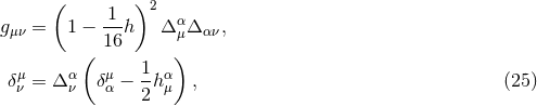
 is the Kronecker delta and
  is defined by the second equation. Indices on
  and
and
 are raised and lowered with
  , but on all other tensors indices are raised and lowered by
  .
Both the Rosen and BSLL bimetric theories give rise to alternative GW polarization states, and have been
used to motivate the construction of the parameterized post-Einsteinian (ppE) waveform families discussed
in Section 5.2.2.
.
Both the Rosen and BSLL bimetric theories give rise to alternative GW polarization states, and have been
used to motivate the construction of the parameterized post-Einsteinian (ppE) waveform families discussed
in Section 5.2.2.
There is also a bimetric theory due to Rastall [374], in which the metric is an algebraic function of the
Minkowski metric and of a vector field  . The action is
![∫ 1 4 [∘ --------- μ;ν ] S = 64-πG- d x − det(g)F(N )K K μ;ν + Smatter, (26 )](article174x.gif)
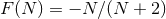 ,
,  and a semicolon denotes a derivative with respect to the
gravitational metric
and a semicolon denotes a derivative with respect to the
gravitational metric  . The metric follows from
  by way of
where
by way of
where 
 is again the non-dynamical flat metric. This theory has not been considered in a GW context
and we will not mention it further; more details, including the field equations, can be found
in [469].
is again the non-dynamical flat metric. This theory has not been considered in a GW context
and we will not mention it further; more details, including the field equations, can be found
in [469].
2.3 The black-hole paradigm
The present consensus is that all of the compact objects observed to reside in galactic centers are supermassive black holes, described by the Kerr metric of GR [377]. This explanation follows naturally in GR from the black-hole uniqueness theorems and from a set of additional assumptions of physicality, briefly discussed below. If a deviation from Kerr is inferred from GW observations, it would imply that the assumptions are violated, or possibly that GR is not the correct theory of gravity. Space-based GW detectors can test black-hole “Kerr-ness” by measuring the GWs emitted by smaller compact bodies that move through the gravitational potentials of the central objects (see Section 6.2). Kerr-ness is also tested by characterizing multiple ringdown modes in the final black hole resulting from the coalescence of two precursors (see Section 6.3).
The current belief that Kerr black holes are ubiquitous follows from work on mathematical aspects of
GR in the middle of the 20th century. Oppenheimer and Snyder demonstrated that a spherically-symmetric,
pressure-free distribution would collapse indefinitely to form a black hole [341]. This result was assumed to
be a curiosity due to spherical symmetry, until it was demonstrated by Penrose [351] and by Hawking and
Penrose [224] that singularities arise inevitably after the formation of a trapped surface during
gravitational collapse. Around the same time, it was proven that the black-hole solutions of
Schwarschild [401] and Kerr [260] are the only static and axisymmetric black-hole solutions in
GR [248, 114, 379]. These results together indicated the inevitability of black-hole formation in
gravitational collapse.
The assumptions that underlie the proof of the uniqueness theorem are that the spacetime is a
stationary vacuum solution, that it is asymptotically flat, and that it contains an event horizon but no
closed timelike curves (CTCs) exterior to the horizon [223]. The lack of CTCs is needed to ensure causality,
while the requirement of a horizon is a consequence of the cosmic-censorship hypothesis (CCH) [352]. The
CCH embodies this belief by stating that any singularity that forms in nature must be hidden behind a
horizon (i.e., cannot be naked), and therefore cannot affect the rest of the universe, which would be
undesirable because GR can make no prediction of what happens in its vicinity. However, the CCH and the
non-existence of CTCs are not required by Einstein’s equations, and so they could in principle be
violated.
Besides the Kerr metric, we know of many other “black-hole–like” solutions to Einstein’s equations: these are vacuum solutions with a very compact central object enclosed by a high-redshift surface. In fact, any metric can become a solution to Einstein’s equation: it is sufficient to insert it in the Einstein tensor, and postulate the resulting “matter” stress-energy tensor as an input to the equations. However, such matter distributions will not in general satisfy the energy conditions (see, e.g., [361]):
- The weak energy condition is the statement that all timelike observers in a spacetime
measure a non-negative energy density,
 , for all future-directed timelike vectors
 . The null energy condition modifies this condition to null observers by replacing
  by
an arbitrary future-directed null vector
by
an arbitrary future-directed null vector  .
.
- The strong energy condition requires the Ricci curvature measured by any timelike observer
to be non-negative,
 , for all timelike
  .
.
- The dominant energy condition is the requirement that matter flow along timelike or null
world lines: that is, that
 be a future-directed timelike or null vector field for any
future-directed timelike vector
be a future-directed timelike or null vector field for any
future-directed timelike vector  .
.
These conditions make sense on broad physical grounds; but even after imposing them, there remain several black-hole–like solutions [427] besides Kerr. Thus, space-based GW detectors offer an important test of the “black-hole paradigm” that follows from GR plus CCH, CTC non-existence, and the energy conditions. This paradigm is especially important: putative black holes are observed to be ubiquitous in the universe, so their true nature has significant implications for our understanding of astrophysics.
If one or many non-Kerr metrics are found, the hope is that observations will allow us to tease apart the various possible explanations:
- Does the spacetime contain matter, such as an accretion disk, exterior to the black hole?
- Are the CCH, the no-CTC assumption, or the energy conditions violated?
- Is the central object an exotic object, such as a boson star [389, 261]?
- Is gravity coupled to other fields? This can lead to different black-hole solutions [265, 396, 413], although some such solutions are known [428]) or suspected [156] to be unstable to generic perturbations.
- Is the theory of gravity just different from GR? For instance, in Chern–Simons gravity black
holes (to linear order in spin) differ from Kerr in their octupole moment [496], and this
correction may produce the most significant observational signature in GW observations [416].
While these questions are challenging, we can learn a lot by testing black-hole structure with space-based GW detectors. These tests are discussed in detail in Section 6.
 |
 |
 |
Living Rev. Relativity, 16 (2013), 7, doi:10.12942/lrr-2013-7, URL (accessed <date>): http://www.livingreviews.org/lrr-2013-7.
 This work is licensed under a Creative Commons License.
© The author(s), except where otherwise noted.
This work is licensed under a Creative Commons License.
© The author(s), except where otherwise noted.