List of Figures
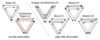 |
Figure 1:
Time-Delay Interferometry (TDI). LISA-like detectors measure GWs by transmitting laser light between three spacecraft in triangular configuration, and comparing the optical phase of the incident lasers against reference lasers on each spacecraft. To avoid extreme requirements on laser-frequency stability over the course of the many seconds required for transmission around the triangle, data analysts will generate time-delayed linear combinations of the phase comparisons; the combinations simulate nearly equal-delay optical paths around the sides of the triangle, and (much like an equal-arm Michelson interferometer) they suppress laser frequency noise. Many such combinations, including those depicted here, are possible, but altogether they comprise at most three independent gravitational-wave observables. Image reproduced by permission from [447], copyright by APS. |
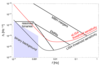 |
Figure 2:
The discovery space for space-based GW detectors, covering the low-frequency region of the GW spectrum,  . The discovery space is delineated by the LISA
threshold sensitivity curve [277] in black, and by the eLISA sensitivity curve in red [21] (the
curves were produced using the online sensitivity curve and source plotting website [321]). This
region is populated by a wealth of strong sources, often in large numbers, including mergers of
MBHs, EMRIs of stellar-scale compact objects into MBHs, and millions of close-orbiting binary
systems in the galaxy. Thousands of the strongest signals from these galactic binary systems should
be individually resolvable, while the combined signals of millions of them produce a stochastic
background at low frequencies. These systems provide ample opportunities for astrophysical tests
of GR for gravitational-field strengths that are not well characterized and studied in conventional
astronomy. . The discovery space is delineated by the LISA
threshold sensitivity curve [277] in black, and by the eLISA sensitivity curve in red [21] (the
curves were produced using the online sensitivity curve and source plotting website [321]). This
region is populated by a wealth of strong sources, often in large numbers, including mergers of
MBHs, EMRIs of stellar-scale compact objects into MBHs, and millions of close-orbiting binary
systems in the galaxy. Thousands of the strongest signals from these galactic binary systems should
be individually resolvable, while the combined signals of millions of them produce a stochastic
background at low frequencies. These systems provide ample opportunities for astrophysical tests
of GR for gravitational-field strengths that are not well characterized and studied in conventional
astronomy. |
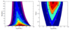 |
Figure 3:
Contours of constant SNR for MBH binaries observed with eLISA. The left-hand panel shows contours in the total-mass–redshift plane for equal-mass binaries, while the right-hand panel shows contours in the total-mass–mass-ratio plane for sources at redshift  . Image reproduced
by permission from [21]. . Image reproduced
by permission from [21]. |
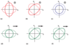 |
Figure 4:
Effect of the six possible GW polarization modes on a ring of test particles. The GW propagates in the z-direction for the upper three transverse modes, and in the x-direction for the lower three longitudinal modes. Only modes (a) and (b) are possible in GR. Image reproduced by permission from [471]. |
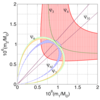 |
Figure 5:
Estimating all the binary-inspiral phasing coefficients  of Eq. (51 of Eq. (51 ) yields differently
shaped regions in the ) yields differently
shaped regions in the  – – plane, which must intersect near true mass values if GR is correct.
Image reproduced by permission from [27], copyright by APS. plane, which must intersect near true mass values if GR is correct.
Image reproduced by permission from [27], copyright by APS. |
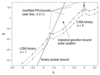 |
Figure 6:
Constraints on phasing corrections in the ppE framework, as determined from LISA observations of  massive–black-hole inspirals at massive–black-hole inspirals at  and and  . The figure also
includes the . The figure also
includes the  bounds derived from pulsar PSR J0737–3039 [492], the solar-system bound on
the graviton mass [435], and PN-coefficient bounds derived as described Section 5.2.1. The spike
at bounds derived from pulsar PSR J0737–3039 [492], the solar-system bound on
the graviton mass [435], and PN-coefficient bounds derived as described Section 5.2.1. The spike
at  corresponds to the degeneracy between the ppE correction and the initial GW-phase
parameter. (Adapted from [134].) corresponds to the degeneracy between the ppE correction and the initial GW-phase
parameter. (Adapted from [134].) |
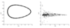 |
Figure 7:
Poincaré map for a regular orbit (left panel) and a chaotic orbit (right panel) in the Manko–Novikov spacetime. Image reproduced by permission from [195], copyright by APS. |
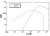 |
Figure 8:
Comparative SNRs, as a function of redshifted black-hole mass  , for the last
year of inspiral of an equal-mass MBH binary and for the ringdown after the merger of the system. The
method used to generate this figure follows that of [182], updated to use a modern LISA sensitivity
curve [277] with a low-frequency cutoff of , for the last
year of inspiral of an equal-mass MBH binary and for the ringdown after the merger of the system. The
method used to generate this figure follows that of [182], updated to use a modern LISA sensitivity
curve [277] with a low-frequency cutoff of  . The redshift is set to . The redshift is set to  , at which
the luminosity distance is , at which
the luminosity distance is  using WMAP 7-year parameters [271]. using WMAP 7-year parameters [271]. |
Jonathan R. Gair and Michele Vallisneri and Shane L. Larson and John G. Baker, "Testing General Relativity with Low-Frequency, Space-Based
Gravitational-Wave Detectors",
Living Rev. Relativity, 16 (2013), 7, doi:10.12942/lrr-2013-7, URL (accessed <date>): http://www.livingreviews.org/lrr-2013-7. This work is licensed under a Creative Commons License.
© The author(s), except where otherwise noted.
This work is licensed under a Creative Commons License.
© The author(s), except where otherwise noted.
Living Rev. Relativity, 16 (2013), 7, doi:10.12942/lrr-2013-7, URL (accessed <date>): http://www.livingreviews.org/lrr-2013-7.
This work is licensed under a Creative Commons License.
© The author(s), except where otherwise noted.