6 Tests of the Nature and Structure of Black Holes
It has become apparent over the last few decades that the centers of most galaxies harbor massive, dark compact objects with masses in the range . It is clear that these objects
play a very important role in the evolution of galaxies. This is exemplified by the very tight
measured correlation (the
. It is clear that these objects
play a very important role in the evolution of galaxies. This is exemplified by the very tight
measured correlation (the  relation) between the mass of the central dark objects and the
velocity dispersion of stars in the central spheroid [174, 441]. It is generally accepted that the
central dark objects are black holes described by the Kerr metric, but there is presently no
definitive proof of that assumption. The alternatives to the black-hole interpretation include dense
star clusters, supermassive stars, magnetoids, boson stars, and fermion balls. Support for the
black-hole interpretation has arisen as a result of both observational and theoretical work. A
short review of the evidence may be found in [115], although we summarize some key details in
Section 6.1.
relation) between the mass of the central dark objects and the
velocity dispersion of stars in the central spheroid [174, 441]. It is generally accepted that the
central dark objects are black holes described by the Kerr metric, but there is presently no
definitive proof of that assumption. The alternatives to the black-hole interpretation include dense
star clusters, supermassive stars, magnetoids, boson stars, and fermion balls. Support for the
black-hole interpretation has arisen as a result of both observational and theoretical work. A
short review of the evidence may be found in [115], although we summarize some key details in
Section 6.1.
As described in Section 2.3, the theoretical basis for the belief that these objects are Kerr black holes
has arisen from proofs that singularities inevitably form during gravitational collapse [341, 351 , 224] and
that the Kerr solution is the unique stationary and axisymmetric black-hole solution in GR [248, 114, 379].
The uniqueness of the Kerr solution is sometimes referred to as the “no-hair” theorem, since the solution is
characterized by just two parameters, the black-hole mass
, 224] and
that the Kerr solution is the unique stationary and axisymmetric black-hole solution in GR [248, 114, 379].
The uniqueness of the Kerr solution is sometimes referred to as the “no-hair” theorem, since the solution is
characterized by just two parameters, the black-hole mass  and angular momentum (per unit mass)
 .
.
The field of any vacuum, axisymmetric spacetime in GR can be characterized by a sequence of mass
and current multipole moments, which we denote as  and
and  respectively [204, 217].
For Kerr spacetimes these multipole moments are all determined by the mass and spin via
respectively [204, 217].
For Kerr spacetimes these multipole moments are all determined by the mass and spin via

6.1 Current observational status
The observational evidence for the presence of black holes in the centers of galaxies has come mainly from
the studies of Active Galactic Nuclei (AGN). These are known to be extremely energetic and also
compact – typical luminosities of  are produced in regions less than
  across [273]. The inferred AGN efficiency of
  10% is much greater than the typical efficiencies of
nuclear fusion processes (
10% is much greater than the typical efficiencies of
nuclear fusion processes ( 1%), implying the need for a very deep relativistic potential. X-ray
observations show variability on timescales of less than an hour, while observations of iron
lines indicate the presence of gas moving at speeds of several thousand km per second [273].
Radio observations of water maser discs are consistent with Keplerian motion around very
compact central objects. In the spiral galaxy NGC 4258 VLBA observations have indicated a disc
with an inner (detected) edge at
1%), implying the need for a very deep relativistic potential. X-ray
observations show variability on timescales of less than an hour, while observations of iron
lines indicate the presence of gas moving at speeds of several thousand km per second [273].
Radio observations of water maser discs are consistent with Keplerian motion around very
compact central objects. In the spiral galaxy NGC 4258 VLBA observations have indicated a disc
with an inner (detected) edge at  0.1 pc, around an object of mass
  [316].
Such compactness cannot be realized by a stellar cluster. In addition, about 10% of AGNs
are associated with jets, which move at highly relativistic velocities and persist for millions of
years. This requires a relativistic potential that has a preferred axis that is stable over very
long timescales. AGNs are also remarkably similar over several decades of mass, which favors
the black-hole explanation, again because Kerr black holes are characterized by just
[316].
Such compactness cannot be realized by a stellar cluster. In addition, about 10% of AGNs
are associated with jets, which move at highly relativistic velocities and persist for millions of
years. This requires a relativistic potential that has a preferred axis that is stable over very
long timescales. AGNs are also remarkably similar over several decades of mass, which favors
the black-hole explanation, again because Kerr black holes are characterized by just  and
and
 .
.
In the Milky Way, evidence for the presence of a black hole coincident with the Sgr A* radio source has
come from observations of stellar motions. These are completely consistent with Keplerian motion around a
point source of mass  [206, 205]. One star, S2, has been observed for one complete orbit
and from this it has been possible to put a limit of 0.066 on the extended fraction of the central mass
that could be contained between pericenter and apocenter of the orbit of S2. At perihelion
S2 was
[206, 205]. One star, S2, has been observed for one complete orbit
and from this it has been possible to put a limit of 0.066 on the extended fraction of the central mass
that could be contained between pericenter and apocenter of the orbit of S2. At perihelion
S2 was  100 AU from the central object, which provides a fairly tight constraint on its
compactness.
100 AU from the central object, which provides a fairly tight constraint on its
compactness.
Electromagnetic observations can rule out stellar clusters as the explanation for the massive central
objects, but some of the exotic alternatives remain. X-ray emission comes from the very inner regions of
accretion discs, but uncertainties in the radius from which the emission is coming and in the mass and spin
of the central object limit their utility for probing the structure of the central object [372]. It is also
possible to construct very compact boson star spacetimes [261] that could not be ruled out from
electromagnetic observations alone. The same applies to spacetimes with a naked singularity. By contrast,
GW observations will probe the spacetime structure as the object proceeds through the inspiral and then
passes the innermost stable orbit and plunges into the horizon of the central object, if a horizon exists. We
discuss the prospects for using GW observations to probe black-hole structure in the following Sections 6.2
and 6.3.
6.2 Tests of black-hole structure using EMRIs
6.2.1 Testing the “no-hair” property
Equation (54 ) tells us that a Kerr black hole is uniquely characterized by two parameters. If we can
measure three multipole moments of the spacetime, we can check that they are consistent with Eq. (54).
If they are not, then the object cannot be a Kerr black hole. Boson stars will typically have
more independent multipole moments. In a certain class of models of rotating boson stars, the
boson star can be uniquely characterized by three multipole moments [389, 73], so a LISA
measurement of four multipole moments could also exclude these models as an explanation of the
data.
) tells us that a Kerr black hole is uniquely characterized by two parameters. If we can
measure three multipole moments of the spacetime, we can check that they are consistent with Eq. (54).
If they are not, then the object cannot be a Kerr black hole. Boson stars will typically have
more independent multipole moments. In a certain class of models of rotating boson stars, the
boson star can be uniquely characterized by three multipole moments [389, 73], so a LISA
measurement of four multipole moments could also exclude these models as an explanation of the
data.
GWs from EMRIs are complicated superpositions of different frequency components, found at harmonics
of the three fundamental frequencies of the orbit: the orbital frequency and the frequencies of
precession of the perihelion and of the orbital plane [154]. This complex structure encodes
detailed information about the spacetime in which the GWs are generated. The details of this
encoding were first worked out by Ryan [387]. If the spacetime is assumed to be stationary and
axisymmetric, it can be shown that the Einstein equations reduce to a single equation, the Ernst
equation, for a complex scalar function, the Ernst potential [165]. By using the Ernst potential and
expressions due to Fodor et al. [183] that relate this potential to the multipole moments of the
spacetime, Ryan was able to study the properties of orbits in vacuum and axisymmetric spacetimes
that possess an arbitrary set of mass and current multipole moments. Circular and equatorial
orbits do not show perihelion or orbital plane precession. However, if such an orbit is given
a small radial or vertical perturbation, it will undergo small oscillations at frequencies (the
“epicyclic” frequencies) that correspond to the perihelion or orbital plane precession frequencies
of nearly circular and nearly equatorial orbits respectively. These frequencies can be readily
computed. For the arbitrary stationary axisymmetric spacetimes considered in [387] one finds
 is the angular (
 ) frequency of the circular orbit being perturbed,
  and
and  are the
perihelion and orbital plane precession frequencies, and
are the
perihelion and orbital plane precession frequencies, and  /
/ denote the mass/current multipole
moments of the spacetime metric, as in Eq. (54). The primary conclusion from Eqs. (55) – (56) is that the
various multipole moments enter the different terms in this expansion at different orders in
denote the mass/current multipole
moments of the spacetime metric, as in Eq. (54). The primary conclusion from Eqs. (55) – (56) is that the
various multipole moments enter the different terms in this expansion at different orders in  . The
precession frequencies and orbital frequency could be extracted from GW observations, so these expansions
are, in principle, observable. We can use this information to “map” the spacetime structure near the central
object and verify that the multipole moments are consistent with the no-hair property (54)
that we expect for a Kerr black hole. This technique is sometimes termed “bothrodesy” or
“holiodesy”5
by analogy with geodesy, in which observations of the motion of satellites are used to probe the
gravitational field of the Earth.
. The
precession frequencies and orbital frequency could be extracted from GW observations, so these expansions
are, in principle, observable. We can use this information to “map” the spacetime structure near the central
object and verify that the multipole moments are consistent with the no-hair property (54)
that we expect for a Kerr black hole. This technique is sometimes termed “bothrodesy” or
“holiodesy”5
by analogy with geodesy, in which observations of the motion of satellites are used to probe the
gravitational field of the Earth.
The multipole moments are also encoded in the total orbital energy lost as the orbital frequency changes by a unit logarithmic interval
A more powerful observable than the three discussed so far is the number of cycles that a trajectory spends near a particular frequency but this is not as clean an observable as the precession frequencies, since it requires computing the rate of energy loss to GWs in an arbitrary spacetime. Ryan used this formalism in conjunction with a post-Newtonian waveform model to estimate LISA’s capability to measure the spacetime multipoles [388
 ].
He considered nearly circular and nearly equatorial inspirals, and found that LISA’s ability to determine the
spacetime multipoles degraded as more multipoles were included in the waveform model. The typical
errors that Ryan found are in Table 3. The conclusion was that LISA would be able to make
moderately accurate measurements of the lowest three multipole moments, but probably no
more.
]. The third
column indicates the highest multipole included in the particular model. Results are shown for two
typical cases, a
].
He considered nearly circular and nearly equatorial inspirals, and found that LISA’s ability to determine the
spacetime multipoles degraded as more multipoles were included in the waveform model. The typical
errors that Ryan found are in Table 3. The conclusion was that LISA would be able to make
moderately accurate measurements of the lowest three multipole moments, but probably no
more.
]. The third
column indicates the highest multipole included in the particular model. Results are shown for two
typical cases, a  inspiral and a
  inspiral; in both cases the SNR
of the inspiral is 10.
inspiral; in both cases the SNR
of the inspiral is 10. |
 |
 |
 |
 |
 |
 |
 |
| 1 | –3.7 | –3.5 | |||||
| 10 | 105 | 2 | –3.0 | –2.9 | –1.8 | ||
| 3 | –2.3 | –1.9 | –1.3 | –0.7 | |||
| 4 | –1.5 | –1.3 | –1.1 | 0.1 | 1.0 | ||
| 1 | –3.3 | –2.8 | |||||
| 10 | 106 | 2 | –2.5 | –1.0 | –0.3 | ||
| 3 | –1.2 | 0.1 | 0.8 | 0.9 | |||
| 4 | –1.0 | 0.1 | 0.8 | 1.2 | 1.8 | ||
Ryan’s analysis was restricted to circular and equatorial orbits, but a counting argument suggests
that spacetime mapping should still be possible for generic orbits [283]. One complication is
that the evolution of the orbital elements must also be inferred from the observation, which
spoils the nice form of the expansions (55) – (56) [195], since all the multipole moments now
enter at each order of the expansion. However, this would also be true if the expansions for
circular-equatorial orbits were rewritten as an expansion in some initial frequency,  , which
would more closely represent a band-limited observation. In practice, the lowest-order multipole
dominates the lowest term in the expansion and so on, which makes spacetime mapping possible in
practice.
, which
would more closely represent a band-limited observation. In practice, the lowest-order multipole
dominates the lowest term in the expansion and so on, which makes spacetime mapping possible in
practice.
The Ryan formalism neatly illustrates why spacetime mapping with EMRIs is possible, but it is not a very practical scheme. We expect that the massive central objects are indeed Kerr black holes and so we really want to consider what imprint small deviations from Kerr will leave on the emitted GWs. A multipole-moment expansion is not a very practical way to do this, as the Kerr metric has an infinite number of nonzero multipoles. Several authors have adopted the approach of constructing spacetimes given by Schwarzschild–Kerr plus a small deviation, and have examined the properties of geodesics in those spacetimes.
Collins and Hughes [125] considered a static deviation from the Schwarzschild metric. This was
constructed by writing the metric in Weyl coordinates and adding a quadrupole perturbation to the
potential (in these coordinates, the potential equation reduces to the flat-space Laplacian for the  cylindrical coordinates, which facilitates writing solutions). They considered two types of quadrupole
perturbation: a torus around the black hole, and the addition of a point mass at each pole. In the second
case, the spacetime necessarily contains line singularities running from the point masses either to infinity or
to the black-hole horizon, which are needed to support the point masses. The solutions are
perturbative, in that the authors kept only the terms that are linear in the deviation from
Schwarzschild. Collins and Hughes explored the properties of orbits in these spacetimes by
comparing the precession and orbital frequencies of equatorial orbits in the spacetime to orbits with
the same orbital parameters in Kerr. They found that there were measurable differences in
the perihelion precession in the strong field: for instance, at a radius of
cylindrical coordinates, which facilitates writing solutions). They considered two types of quadrupole
perturbation: a torus around the black hole, and the addition of a point mass at each pole. In the second
case, the spacetime necessarily contains line singularities running from the point masses either to infinity or
to the black-hole horizon, which are needed to support the point masses. The solutions are
perturbative, in that the authors kept only the terms that are linear in the deviation from
Schwarzschild. Collins and Hughes explored the properties of orbits in these spacetimes by
comparing the precession and orbital frequencies of equatorial orbits in the spacetime to orbits with
the same orbital parameters in Kerr. They found that there were measurable differences in
the perihelion precession in the strong field: for instance, at a radius of  for a 2%
perturbation of the black hole, the trajectory would accumulate one radian of dephasing in
for a 2%
perturbation of the black hole, the trajectory would accumulate one radian of dephasing in  1000
orbits. Collins and Hughes coined the term “bumpy black hole” to describe spacetimes of this
type.
1000
orbits. Collins and Hughes coined the term “bumpy black hole” to describe spacetimes of this
type.
Glampedakis and Babak [207] took a different approach to studing deviations from Kerr. Starting from
the Hartle–Thorne metric [220, 221], which is an exact solution to Einstein’s equations describing the
spacetime outside of a slowly, rigidly rotating axisymmetric object, the authors constructed a spacetime
with metric of the form  , working perturbatively and keeping only
the
, working perturbatively and keeping only
the  perturbation in the quadrupole mass moment. They termed the resulting spacetime a
“quasi-Kerr” solution. A comparison of the frequencies of eccentric equatorial geodesics in the
quasi-Kerr spacetime to the same geodesics in the Kerr spacetime indicated that it would take only
perturbation in the quadrupole mass moment. They termed the resulting spacetime a
“quasi-Kerr” solution. A comparison of the frequencies of eccentric equatorial geodesics in the
quasi-Kerr spacetime to the same geodesics in the Kerr spacetime indicated that it would take only
 100 cycles to accumulate a
  phase shift for a
  1% deviation from Kerr. They also
computed waveform overlaps and found that, over the radiation-reaction timescale, the overlap
of the waveforms for an orbit with a semilatus rectum of ten geometric radii (
1% deviation from Kerr. They also
computed waveform overlaps and found that, over the radiation-reaction timescale, the overlap
of the waveforms for an orbit with a semilatus rectum of ten geometric radii ( ) was
) was
 20%, 50%, 90%, 98% for inspirals with mass ratio
  ,
,  ,
,  ,
,  respectively.
A third approach to analyzing deviations from the Kerr spacetime was considered by Gair et al. [195],
who studied geodesic motion in a family of exact spacetimes due to Manko and Novikov [303], which
include the Kerr spacetime for a specific choice of parameters. By using exact solutions of the Einstein field
equations, they obtained solutions that were valid everywhere, in contrast to the perturbative solutions
considered in [125, 207], which break down near the central object. However, this scheme offers less control
over the multipole moments, since it is possible to choose the lowest multipole that differs from Kerr, but
then the higher multipoles must also change. Gair et al. [195] studied observable properties of the orbits,
including the variation of the precession frequencies of nearly circular and nearly equatorial
orbits as a function of orbital frequency, and the loss of the third integral of the motion (see
Section 6.2.5).
These three papers outlined different ways to approach the problem of spacetime mapping in practice.
However, none of the analyses were complete as they did not consider inspirals. Collins and Hughes and
Glampedakis and Babak also ignored waveform confusion by assuming that the orbital elements were the
same between the orbits under consideration. Glampedakis and Babak did discuss the importance of
confusion and the role of the inspiral evolution in breaking such degeneracies, but no inspiral results were
included in the published paper. Observationally, the correct orbits to compare will be those with the same
frequencies since we have no way to determine the orbital radius or eccentricity directly. This was the
approach adopted in [195]. Assessing the confusion problem is relatively easy, but including inspiral is
very hard in general, since the presence of excess multipole moments in the spacetime leads to
changes in the rates of energy and angular momentum loss, which must also be included in
the analysis. Progress can be made in the presence of small deviations by including only the
leading-order contributions to the radiation reaction from the multipole moments. This is an open
area of research, although Barack and Cutler [47] carried out a preliminary assessment using
post-Newtonian EMRI waveforms [46] augmented with the leading-order contribution of an
excess quadrupole moment to the precession and inspiral rates. The resulting waveforms were an
improvement in comparison to Ryan’s analysis [388], since they included orbital eccentricity
and inclination, and were filtered through an approximation of the LISA response. Barack and
Cutler performed a Fisher-matrix analysis of parameter-estimation uncertainties, and hence
correctly accounted for the confusion issue. For this simple model, they found that a single LISA
observation of the inspiral of a  black hole into a
  ,
,  or
or  black hole could measure the deviation from Kerr of the quadrupole moment to an accuracy of
 , while simultaneously measuring the mass and spin of the central object to
fractional accuracies of
, while simultaneously measuring the mass and spin of the central object to
fractional accuracies of  . This suggests that a LISA-like observatory would be able to perform
high-precision tests of the no-hair property of massive compact objects in galactic centers.
To put these numbers in perspective, a boson star may have a quadrupole moment that is
. This suggests that a LISA-like observatory would be able to perform
high-precision tests of the no-hair property of massive compact objects in galactic centers.
To put these numbers in perspective, a boson star may have a quadrupole moment that is
 times that of a Kerr black hole with the same mass and spin [389], so it could easily be
excluded.
times that of a Kerr black hole with the same mass and spin [389], so it could easily be
excluded.
6.2.2 Probing the nature of the central object
During an EMRI, the inspiraling object interacts gravitationally with the horizon of the central black hole.
This can be thought of as a tidal interaction – the gravitational field of the small body raises a tide on the
horizon that is dragged around through the orbit, leading to dissipation of energy – or as energy being lost
by GWs falling into the black hole. Fang and Lovelace [170] explored the nature of the tidal-coupling
interaction by perturbing a Schwarzschild black hole with a distant orbiting moon. They found
that the time-dependent piece of the perturbation affected the orbit in an unambiguous way: a
time-varying quadrupole moment is induced on the black-hole horizon that is proportional to the
time derivative of the moon’s tidal field. This quadrupole perturbation extracts energy and
angular momentum from the orbit at the same rate that energy and angular momentum enter
the horizon. However, the effect of the time-independent piece of the perturbation remained
ambiguous. Working in the Regge–Wheeler gauge, Fang and Lovelace found that this piece vanished,
in contrast to a previous result by Suen [432], who used a different gauge. This ambiguity
leads to an ambiguity in the phase of the induced quadrupole moment as measured in a local
asymptotic rest frame (LARF), although the phase of the bulge relative to the orbiting moon is
well defined (using a spacelike connection between the moon and the black hole, Fang and
Lovelace found that the horizon shear led the horizon tidal field by an angle of  , where
  is the angular velocity of the moon). The ambiguity of interpretation in the LARF makes it
impossible to define the polarizability of the horizon or the phase shift of the tidal bulge in a
body-independent way. Fang and Lovelace left open the possibility of developing a body-independent
language to describe the response of the central object to tidal coupling, but as yet this has not
happened.
is the angular velocity of the moon). The ambiguity of interpretation in the LARF makes it
impossible to define the polarizability of the horizon or the phase shift of the tidal bulge in a
body-independent way. Fang and Lovelace left open the possibility of developing a body-independent
language to describe the response of the central object to tidal coupling, but as yet this has not
happened.
Although the nature of the response of the central object to tidal coupling may be difficult to
characterize from GW observations, the total energy lost to tidal interactions is a good observable.
Ryan’s original theorem [387] ignored tidal coupling, but it was later generalized by Li and
Lovelace [283]. They found that the GWs propagating to infinity depended only very weakly
on the inner boundary conditions (i.e., on the nature of the central object). This means that
the spacetime’s multipole structure can be inferred from the outgoing radiation field in the
usual way, and hence the expected rate of orbital energy loss, assuming no energy loss into
the central body, can be calculated. The rate of inspiral measures the actual rate of orbital
energy loss, and the difference then gives the rate at which energy is lost to the central object,
which is a direct measure of the tidal coupling. Li and Lovelace estimated that the ratio of
the change in energy radiated to infinity due to the inner boundary condition to the energy
in tidal coupling scales with the orbital velocity as  . Therefore, it should be possible to
simultaneously determine the spacetime structure and the tidal coupling through low-frequency GW
observations.
. Therefore, it should be possible to
simultaneously determine the spacetime structure and the tidal coupling through low-frequency GW
observations.
Information about the central object can also come from the transition to plunge at the end of the
inspiral. In a black-hole system, we expect GW emission to cut off sharply as the orbit reaches the
innermost stable orbit and then plunges rapidly through the horizon. If there is no horizon in the system,
the orbit may instead enter a phase where it passes into and out of the material of the central object. This
was explored for boson-star models in [261]: Kesden et al. found that persistent radiation after the
apparent innermost orbit could be a clear signature of the presence of a supermassive, horizonless central
object in the spacetime. This analysis did not treat gravitational radiation or the interaction of the
inspiraling body with the central object accurately, but it does illustrate a possible way to
identify non–black-hole central objects. Something similar might happen if the spacetime were
to contain a naked singularity rather than a black hole [195]: in principle, the nature of the
emitted waveform after “plunge” would encode information about the exact nature of the central
object. However, this has not yet been investigated. Naked-singularity spacetimes may have
very–high-redshift surfaces rather than horizons: these spacetimes would be observationally
indistinguishable from black holes, unless the inspiraling object happened to move inside the
high-redshift surface and then emerged, and the two epochs of radiation could be connected
observationally.
Another example of an object that can be arbitrarily close to a Schwarzschild black hole in the exterior but lack a horizon is a gravastar [346]. These are constructed by matching a de Sitter spacetime interior onto a Schwarzschild exterior through a thin shell of matter, whose radius can be made arbitrarily close to the Schwarzschild horizon. It was shown in [346] that the oscillation modes of such a gravastar have quasinormal frequencies that are completely different from those of a Schwarzschild black hole. Therefore the absence of a horizon would be apparent if ringdown radiation was observed from such a system. In addition, the tidal perturbations that arise during the inspiral of a compact object into a gravastar during an EMRI [347] can resonantly excite polar oscillations of the gravastar as the orbital frequency passes through certain values over the course of the inspiral. The excitation of these modes generates peaks in the GW-emission spectrum at frequencies that are characteristic of the gravastar, and can also show signatures of the microscopic surface of the gravastar. This process would be apparent both in the amplitude of the detected GWs and in the rate of inspiral inferred from the gravitational-waveform phase, since the rate of inspiral will change significantly in the vicinity of each resonance due to the additional energy radiated in the excited quasi-normal modes. Although the gravastar model used in [346, 347] may not be physically relevant, this work illustrates the more general fact that if the horizon of a black hole is replaced by some kind of membrane, then the modes of that membrane will inevitably be excited during an inspiral and these modes will typically be different to those of a black hole.
6.2.3 Astrophysical perturbations: the influence of matter
A change in the inspiral trajectory need not be caused only by differences in the central object, but might arise due to the presence of material in the spacetime, close to the black hole but external to the event horizon. Such material could influence the inspiral trajectory, and hence the emitted GWs, in two distinct ways: the gravitational field of the matter could modify the multipole moments of the spacetime and hence the orbit as discussed above; if the orbital path intersected the material, it would cause sufficient hydrodynamic drag on the object to alter the orbit.The influence of the gravitational field of external material was considered in [53]: Barausse et al. constructed a model spacetime that included both a black hole and an external torus of material very close to the central black hole. They examined the properties of orbits in two systems: one with a torus of comparable mass and spin to the central black hole (spacetime “A”), and one with a torus of low mass, but much greater angular momentum than the central black hole (spacetime “B”). Their comparisons were based on computing equatorial geodesics and then “kludge” gravitational waveforms in the spacetime and in a corresponding Kerr spacetime, and then evaluating the waveform overlap. Orbits were identified by matching the radial and azimuthal frequencies between the orbits in the two spacetimes in two ways: altering the orbital parameters, while setting the mass and spin to be the same in the corresponding Kerr spacetime; or altering the mass and spin, while keeping the orbital parameters the same.
This approach identified a confusion problem: over much of the parameter space the overlaps were very high, particularly when the second approach was adopted. Overlaps were lower in spacetime “B” than in spacetime “A,” and overlaps for “internal” orbits between the black hole and the torus were particularly low. This work suggested that it would not be possible to distinguish between such a spacetime and a pure Kerr spacetime in low-frequency GW EMRI observations. However, it did not consider inspiraling orbits. The need to constantly adjust the orbital parameters in order to maintain equality of frequencies would lead to a difference in the evolution of the orbit between the two spacetimes, which might break the waveform degeneracies. The torus model was also not physical, being much more compact than one would expect for AGN discs.
The effect of hydrodynamic drag on an EMRI was first considered in [326] and was found to be negligibly small for systems likely to be of interest to space-based gravitational-wave detectors. The problem was revisited in [52]: Barausse and Rezzolla considered a spacetime containing a Kerr black hole surrounded by a non–self-gravitating torus with constant specific angular momentum. The hydrodynamic drag consists of a short-range part that arises from accretion, and a long-range part that arises from the gravitational interaction of the body with the density perturbations it causes in the disc. The accretion onto the small object was modeled as Bondi–Hoyle–Lyttleton accretion6 and the long-range force using collisional dynamical-friction results from the literature [264, 50]. The effect of the hydrodynamical drag on the orbital evolution was computed for geodesic orbits and compared to the orbital evolution from radiation reaction for a variety of torus models, varying in mass and outer radius.
The conclusion was that, for realistic outer radii for the torus,  , the effect of
hydrodynamic drag on the orbital radius and eccentricity was always small compared to radiation
reaction. However, the relative importance increases further from the central black hole. The
hydrodynamic drag has a greater relative effect on the orbital inclination, and tends to cause orbits to
become more prograde, which is opposite to the effect of radiation reaction. For
, the effect of
hydrodynamic drag on the orbital radius and eccentricity was always small compared to radiation
reaction. However, the relative importance increases further from the central black hole. The
hydrodynamic drag has a greater relative effect on the orbital inclination, and tends to cause orbits to
become more prograde, which is opposite to the effect of radiation reaction. For  ,
the hydrodynamic drag becomes significant at
,
the hydrodynamic drag becomes significant at  , but this radius is smaller for a
more compact torus. Thus, this effect will only be important for LISA if we observe a system
with a very compact accretion torus, or for systems of low central mass. For the latter, the
GWs are detectable from orbits at larger radii where hydrodynamic drag can be important.
However, the SNR of such events will be low, so we are unlikely to see many of them [192]. Thus,
although it seems that this effect is also marginal, this conclusion is based on considering geodesic
orbits, and the possible secular build up of a drag signature over the inspiral has yet to be
examined,
, but this radius is smaller for a
more compact torus. Thus, this effect will only be important for LISA if we observe a system
with a very compact accretion torus, or for systems of low central mass. For the latter, the
GWs are detectable from orbits at larger radii where hydrodynamic drag can be important.
However, the SNR of such events will be low, so we are unlikely to see many of them [192]. Thus,
although it seems that this effect is also marginal, this conclusion is based on considering geodesic
orbits, and the possible secular build up of a drag signature over the inspiral has yet to be
examined,
The influence of an accretion disc on the evolution of an EMRI embedded within it was explored
in [493, 268]. One of the channels that has been suggested to produce EMRIs is the formation of stars in a
disc, followed by the capture of the compact stellar remnants left after the evolution of those
stars [18, 16]. The migration of such an EMRI through the accretion disc could potentially leave a
measurable imprint on the GW signal. The literature distinguishes between two types of migration.
In Type I migration, which generally occurs for lower-mass objects, the disc persists in the
vicinity of the object throughout the inspiral. The object excites density waves in the disc,
which exert a torque on the object. In general, the torque from material exterior to the orbit is
greater than that from material interior to the orbit, which causes the object to lose angular
momentum and spiral inward on a timescale that is short relative to the lifetime of the disc. In
Type II migration, a gap opens in the disc in the vicinity of the inspiraling object. Material
enters the gap on the disc’s accretion timescale, driving the object and gap inwards on that
timescale.
Yunes, Kocsis et al. [493, 268] considered migration in geometrically-thin and radiatively-efficient discs,
in which thermal energy is radiated on a much shorter timescale than the timescale over which the material
moves inward, so the disc can remain thin. Such discs can be described by the Shakura–Sunyaev  -disc
model [409], in which the viscous stress in the disc is proportional to the total pressure at each point in the
disc. These discs are known to be unstable to linear perturbations [286, 410, 83, 358]. The alternative
-disc
model [409], in which the viscous stress in the disc is proportional to the total pressure at each point in the
disc. These discs are known to be unstable to linear perturbations [286, 410, 83, 358]. The alternative
 -disc model, where stress is proportional to the gas pressure only, is stable to perturbations [391]. Both
disc models were considered for EMRI migration. Yunes, Kocsis et al. showed that, over a year of
observation, Type I migration could lead to
-disc model, where stress is proportional to the gas pressure only, is stable to perturbations [391]. Both
disc models were considered for EMRI migration. Yunes, Kocsis et al. showed that, over a year of
observation, Type I migration could lead to  radian dephasings in an EMRI signal for both
 -discs and
  -discs, while Type II migration could lead to dephasings of
  radians.
The effects are larger for
radians.
The effects are larger for  discs, since these can support higher surface density. For more
massive central black holes
discs, since these can support higher surface density. For more
massive central black holes  the dominant contribution is from Bondi–Hoyle accretion
(see Footnote 6 for a description), while for less massive black holes of
the dominant contribution is from Bondi–Hoyle accretion
(see Footnote 6 for a description), while for less massive black holes of  the
dominant contribution is from the migration. These dephasings were computed for the same system
parameters (apart from maximizing over time and phase shifts), so they do not account for possible
parameter correlations, but the authors argue that the migration dephasing decouples from
GW parameters as the effect becomes weaker with decreasing orbital radius, while relativistic
effects become stronger. The relative number of EMRIs that will be produced in discs rather
than from other channels is not well understood. However, it will be straightforward to identify
such EMRIs, which will be circular and equatorial, to look for and constrain effects of this
type.
the
dominant contribution is from the migration. These dephasings were computed for the same system
parameters (apart from maximizing over time and phase shifts), so they do not account for possible
parameter correlations, but the authors argue that the migration dephasing decouples from
GW parameters as the effect becomes weaker with decreasing orbital radius, while relativistic
effects become stronger. The relative number of EMRIs that will be produced in discs rather
than from other channels is not well understood. However, it will be straightforward to identify
such EMRIs, which will be circular and equatorial, to look for and constrain effects of this
type.
Another important question that has not yet been addressed is how to distinguish the effect of external material from a difference in the structure of the central object. If the orbit does not intersect the material, such identification would come from the variation in the effect over the inspiral – if the change in the multipole structure comes from material, then at some stage the object would pass inside the matter, and the qualitative effect on the inspiral would be different from that of a central object with an unusual multipole structure. If the orbit does intersect the material, then the spacetime-mapping analysis described above no longer applies, since the Geroch–Hansen multipole decomposition [204, 217] applies to vacuum spacetimes only. If this decomposition could be generalized to nonvacuum axisymmetric spacetimes, then low-frequency GW observation could potentially recover not only the spacetime metric but also the structure of the external material. It would then be possible to verify that this matter obeys the various energy conditions (see Section 2.3). This is an open area of research at present.
An independent indicator of the presence of material in the spacetime would come from the observation
of an electromagnetic counterpart to an EMRI event. For instance, if an inspiraling black hole was moving
through an accretion disc, there might be emission from the material that was accreted onto the inspiraling
object or from shocks formed in the disc. Again, this has not been explored, although it is likely, given the
poor sky-position determination of EMRI events in GW observations [46], that it would not be
possible to conclusively identify such a weak electromagnetic signature in coincidence with a GW
event.
The presence of exotic matter outside a black hole, in the form of a cloud of axions, was discussed in [34]. The presence of large numbers of light axions would be one consequence of extra dimensions in string theory, so the detection of an axion cloud would provide strong evidence in support of their existence. The axion cloud would modify the motion of an inspiraling black hole in a similar way to regular matter, although estimates for the precision of measurements possible with future GW detectors have not yet been carried out. The passage of an EMRI through the cloud could also lead to its disruption, which may rule out the cloud as a possible explanation for any observed deviations, but further theoretical work is required to properly quantify these processes.
The existence of axion clouds can also have other observable GW signatures. The axions in the cloud
exist in different quantum energy states. If multiple states with the same orbital momenta  and magnetic
moments
and magnetic
moments  but different principal quantum numbers
  are occupied, transitions between these states
can generate GWs with characteristic strain
are occupied, transitions between these states
can generate GWs with characteristic strain

 at a distance
  . The pre-factor
  depends on the axion masses
and coupling. The axions can also undergo annihilations, which generate GWs with very similar
characteristic strains
In both cases the frequency depends on the black-hole mass in the usual way
depends on the axion masses
and coupling. The axions can also undergo annihilations, which generate GWs with very similar
characteristic strains
In both cases the frequency depends on the black-hole mass in the usual way 
 , with typical
values for
, with typical
values for  black holes of
  and
and  respectively. Both eLISA and LIGO
could place interesting constraints on the axion parameter space through (non)detections of
these events [34]. Finally, the self-interactions in the axion cloud could eventually lead to the
collapse of the cloud in a “bosenova” explosion [269, 489], which would generate GWs with strain
and frequency
respectively. Both eLISA and LIGO
could place interesting constraints on the axion parameter space through (non)detections of
these events [34]. Finally, the self-interactions in the axion cloud could eventually lead to the
collapse of the cloud in a “bosenova” explosion [269, 489], which would generate GWs with strain
and frequency 
 . These could also be an interesting source for low-frequency GW detectors.
Recent calculations [489] suggest that a bosenova from the Milky Way black hole at Saggitarius A* would
be marginally detectable by LISA. The bosenova explosion comes about due to a super-radiant interaction
between the cloud of particles and the central black hole, which extracts rotational energy from the black
hole and transfers it to the cloud of particles. Recent results on these super-radiant instabilities can be
found in [479].
. These could also be an interesting source for low-frequency GW detectors.
Recent calculations [489] suggest that a bosenova from the Milky Way black hole at Saggitarius A* would
be marginally detectable by LISA. The bosenova explosion comes about due to a super-radiant interaction
between the cloud of particles and the central black hole, which extracts rotational energy from the black
hole and transfers it to the cloud of particles. Recent results on these super-radiant instabilities can be
found in [479].
In [297] the observable signatures of the presence of a cloud of bosons outside a massive compact object was considered. It was shown that the motion of a particle through the cloud would be dominated by boson accretion rather than by gravitational radiation reaction. During this accretion-dominated phase, the frequency and amplitude of the gravitational-wave emission is nearly constant in the late stages of inspiral. The authors also considered inspirals exterior to the boson cloud, and found that resonances could occur when the orbital frequency matched the characteristic frequency associated with the characteristic mass of the bosonic particles. These resonances could lead to significant, detectable deviations in the phase of the emitted GWs.
6.2.4 Astrophysical perturbations: distant objects
Perturbations to the EMRI trajectory could also arise from the gravitational influence of distant objects, such as other stars or a second MBH. At present, it is thought to be very unlikely that a second star or compact object would be present in the spacetime sufficiently close to the EMRI to leave a measurable imprint on the trajectory [18], although detailed calculations for this scenario have not been carried out.
However, if the MBH that was the host of the EMRI was in a binary with a second MBH, this
could perturb the trajectory by a detectable amount [494]. The primary observable effect is a
Doppler shift of the GW signal, which arises due to the acceleration of the center of mass of the
EMRI system relative to the observer. It was estimated that, for typical EMRI systems, the
presence of a second black hole within a few tenths of a parsec would lead to a measurable
imprint in the signal. The frequency scaling of the Doppler effect differs from the scaling of the
post-Newtonian terms in the unaccelerated waveform, which suggests that this effect will be
distinguishable in GW observations [494]. The magnitude of the leading-order Doppler effect scales as
 , where
  is the mass of the perturbing black hole, and
  is its distance. If the
second object is within a few hundredths of a parsec, higher-order time derivatives could also
be measured from the GW observations. These scale differently with
is its distance. If the
second object is within a few hundredths of a parsec, higher-order time derivatives could also
be measured from the GW observations. These scale differently with  and
and  , which
would in principle allow the mass and distance of the perturber to be measured from the EMRI
data [494].
, which
would in principle allow the mass and distance of the perturber to be measured from the EMRI
data [494].
The probability that a second black hole would be within a tenth of a parsec of a system containing an
EMRI is difficult to assess. At redshifts  , at any given time a few percent of Milky Way-like galaxies
will be involved in a merger, which suggests an upper limit of a few percent of EMRIs that could have
perturbing companions. However, there is uncertainty as to how long the black-hole binary will spend at
radii of a few tenths of a parsec following a merger, and it is plausible that the presence of a second black
hole would increase the EMRI rate by perturbing stars onto orbits that pass close to the other black hole,
introducing an observational bias in favor of these systems [494]. Given these uncertainties, the possibility
of a distant perturber will have to be accounted for in the analysis, and, if it is observed in
some systems, LISA-like detectors could indirectly inform us of the processes that drive MBH
mergers.
, at any given time a few percent of Milky Way-like galaxies
will be involved in a merger, which suggests an upper limit of a few percent of EMRIs that could have
perturbing companions. However, there is uncertainty as to how long the black-hole binary will spend at
radii of a few tenths of a parsec following a merger, and it is plausible that the presence of a second black
hole would increase the EMRI rate by perturbing stars onto orbits that pass close to the other black hole,
introducing an observational bias in favor of these systems [494]. Given these uncertainties, the possibility
of a distant perturber will have to be accounted for in the analysis, and, if it is observed in
some systems, LISA-like detectors could indirectly inform us of the processes that drive MBH
mergers.
The gravitational influence of a second stellar mass black hole on the evolution of an EMRI were
considered in [17]. It was shown that a second black hole with a semi-major axis of  could
influence the orbital parameters of an EMRI ongoing in the same galaxy and already in the
low-frequency GW band. This influence is chaotic, leading to an unpredictable evolution of the orbital
parameters. It was estimated that in 1% of EMRIs a second black hole could be within the required
distance. However, the timescale of the chaotic motion was
could
influence the orbital parameters of an EMRI ongoing in the same galaxy and already in the
low-frequency GW band. This influence is chaotic, leading to an unpredictable evolution of the orbital
parameters. It was estimated that in 1% of EMRIs a second black hole could be within the required
distance. However, the timescale of the chaotic motion was  , which is much longer than a
typical low-frequency observation, and the system considered in [17] had an orbital period
of
, which is much longer than a
typical low-frequency observation, and the system considered in [17] had an orbital period
of  , which would probably not yet be detectable by LISA-like detectors. On the
timescale of a GW mission, the effect would probably manifest itself as a linear drift in the
orbital parameters, and therefore it is unlikely that this effect would prevent the detection of an
EMRI signal. A full analysis of the effect on parameter estimation has not yet been carried
out.
, which would probably not yet be detectable by LISA-like detectors. On the
timescale of a GW mission, the effect would probably manifest itself as a linear drift in the
orbital parameters, and therefore it is unlikely that this effect would prevent the detection of an
EMRI signal. A full analysis of the effect on parameter estimation has not yet been carried
out.
6.2.5 Properties of the phase space of orbits
Loss of the third integral.
It was demonstrated by Carter [113] that the Kerr metric has a complete set of integrals – in addition to
the energy and angular momentum that arise as conserved quantities in any stationary and axisymmetric
spacetime, geodesics in the Kerr metric conserve the Carter constant,  . This is the analog of
the third isolating integral found in some classical axisymmetric systems, and has been shown
to arise due to the existence of a Killing tensor of the spacetime [463]. In the Schwarzschild
limit,
. This is the analog of
the third isolating integral found in some classical axisymmetric systems, and has been shown
to arise due to the existence of a Killing tensor of the spacetime [463]. In the Schwarzschild
limit,  is the sum of the squared angular momentum components in the two equatorial
directions. The Kerr metric is one of a very special class of metrics that have this property. In fact,
Carter [113] demonstrated that it was the only axisymmetric metric not containing a gravitomagnetic
monopole for which both the Hamilton–Jacobi and Schrödinger equations were separable. The
special nature of the Kerr metric was emphasized by Will [472] who demonstrated that, in
Newtonian gravity, motion about a body with an arbitrary set of multipole moments
is the sum of the squared angular momentum components in the two equatorial
directions. The Kerr metric is one of a very special class of metrics that have this property. In fact,
Carter [113] demonstrated that it was the only axisymmetric metric not containing a gravitomagnetic
monopole for which both the Hamilton–Jacobi and Schrödinger equations were separable. The
special nature of the Kerr metric was emphasized by Will [472] who demonstrated that, in
Newtonian gravity, motion about a body with an arbitrary set of multipole moments  possesses a third integral of the motion only if the multipole moments obey the conditions
which are precisely the conditions satisfied by the mass moments of a Kerr black hole, Eq. (54
possesses a third integral of the motion only if the multipole moments obey the conditions
which are precisely the conditions satisfied by the mass moments of a Kerr black hole, Eq. (54 ).
).
The separability of the Kerr metric aids the analysis of inspirals in that spacetime, but it also suggests
another potential observable that would show a deviation from the Kerr metric in a GW observation. The
specialness of the third integral in the Kerr spacetime suggests that if a spacetime differed from the Kerr
solution, even by a small amount, the third integral might vanish, which would potentially lead to the
existence of chaotic orbits. If such orbits were observed it would be a clear “smoking gun” for a deviation
from the Kerr metric. The existence of chaotic orbits in various spacetimes has been explored by several
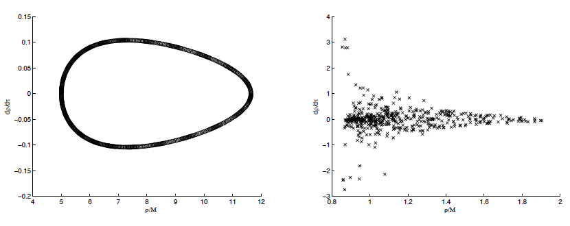
authors. The standard approach is via construction of a Poincaré map: a geodesic is computed in
cylindrical coordinates  , and the values of
  and
and  recorded every time the particle
intersects a specified plane
recorded every time the particle
intersects a specified plane  = constant. If the resulting plot of all these points on a (
 ) plane yields
a closed curve, then a third integral exists, otherwise the orbit is chaotic. This is illustrated in
Figure 7
) plane yields
a closed curve, then a third integral exists, otherwise the orbit is chaotic. This is illustrated in
Figure 7 .
.
 ], copyright by APS.
 Chaotic motion has been found by Sota et al. for orbits in the Zipoy–Voorhees–Weyl and Curzon
spacetimes [417]; by Letelier and Viera for orbits around a Schwarzschild black hole perturbed by
GWs [282]; by Guéron and Letelier for orbits in a black-hole spacetime with a dipolar halo [213],
and in prolate Erez–Rosen bumpy spacetimes [214]; and by Dubeibe et al. for some oblate
spacetimes that are deformed generalizations of the Tomimatsu–Sato spacetime [157]. None of
these examples represented systems that were small deviations from the Kerr metric. The only
investigation to date of chaotic orbits in the context of LISA was by Gair et al. [195], who explored
geodesic motion in a family of spacetimes due to Manko and Novikov [303] that had arbitrary
multipole moments, but which included Kerr as a special case. Gair et al. [195] considered orbits
in a family of spacetimes parameterized by a single “excess quadrupole moment” parameter,
 , such that
  represented the Kerr solution. They found that, while the majority
of orbits in these spacetimes possessed an apparent third integral, chaotic orbits existed very
close to the central object for arbitrarily small oblate deformations of the Kerr solution. As the
spacetime was deformed away from Kerr, a second allowed region for bound geodesic motion
was found to appear close to the central black hole, in addition to the allowed region present
in the Kerr metric. Chaotic orbits were found only in this additional bound region. Gair et
al. [195] concluded that this chaotic region would probably be inaccessible to an object that was
initially captured at a large distance from the central object. This analysis was revisited in [294]
but the conclusions in that paper were the same. The only difference was that the authors
in [294] identified a region of stable motion within the inner region that contains chaotic orbits.
The chaotic orbit shown in the right hand panel of Figure 7 appears to pass in and out of the
region of stability which should not happen, so this might be a numerical artifact. However, the
existence of chaotic orbits and the probable inaccessibility of these orbits to inspirals was confirmed
by [294].
represented the Kerr solution. They found that, while the majority
of orbits in these spacetimes possessed an apparent third integral, chaotic orbits existed very
close to the central object for arbitrarily small oblate deformations of the Kerr solution. As the
spacetime was deformed away from Kerr, a second allowed region for bound geodesic motion
was found to appear close to the central black hole, in addition to the allowed region present
in the Kerr metric. Chaotic orbits were found only in this additional bound region. Gair et
al. [195] concluded that this chaotic region would probably be inaccessible to an object that was
initially captured at a large distance from the central object. This analysis was revisited in [294]
but the conclusions in that paper were the same. The only difference was that the authors
in [294] identified a region of stable motion within the inner region that contains chaotic orbits.
The chaotic orbit shown in the right hand panel of Figure 7 appears to pass in and out of the
region of stability which should not happen, so this might be a numerical artifact. However, the
existence of chaotic orbits and the probable inaccessibility of these orbits to inspirals was confirmed
by [294].
Brink [94] also explored integrability in arbitrary stationary, axisymmetric and vacuum spacetimes,
concentrating on regions where the Poincaré maps indicated the presence of an effective third
integral. Brink hypothesized that some spacetimes might admit an integral of the motion that
was quartic in the momentum, in contrast to the Carter constant, which is quadratic. This
hypothesis is as yet unproven. There is also a potential conflict with the example given in [195]. The
Kolmogorov, Arnold, and Moser (KAM) theorem indicates that when a Hamiltonian system
with a complete set of integrals is weakly perturbed, the phase-space motion will either be
confined to the neighborhoods of the invariant tori, or the motion will be chaotic [434]. Thus, if
there is a region of the spacetime where chaotic motion exists, there cannot be another region
where a third invariant exists. A mathematical demonstration that the orbits can possess an
approximate invariant, while technically being chaotic, is lacking at present, although this does
appear to be the case from the numerical calculations [195]. It is also not entirely clear that the
perturbation can be regarded as “small” everywhere, since the change in mutipole moments
necessarily changes the horizon structure and so the perturbation is infinitely large at certain
points.
A discussion of the reason for the existence of chaotic geodesics in some spacetimes was given by Sota et
al. [417]. They suggested that it would arise either from a change in sign of the eigenvalues of the Weyl
tensor at a point, which would lead to a local “instability,” or from the existence of homoclinic orbits. The
latter explanation applied only to non-reflection-symmetric spacetimes, while most spacetimes of
astrophysical interest should be reflection symmetric. The Weyl-tensor analysis has not been carried out for
the Manko–Novikov family of spacetimes [195]. One other proposed explanation was the existence of a
region of closed timelike curves, which was found to touch the region in which chaotic motion was
identified [195].
In conclusion, it seems unlikely that chaotic geodesics will be found in nature, but if they were identified
we would know immediately that the spacetime was not Kerr. However, detecting chaotic motion from a
GW observation is challenging. One possibility would be to observe the transition from regular to chaotic
motion in a time-frequency analysis: the regular motion would be characterized by a few well-distinguished
peaks in a Fourier transform of the signal, while chaotic motion would show a much broader band
structure [195]. However, it is not clear that it would be possible to distinguish the chaotic phase from
detector noise, and hence there would be no way to identify an inspiral that “ends” by entering a chaotic
phase as opposed to one which ends at plunge into a black hole. If an orbit passed into a chaotic
phase and then back into a regular phase we might see a signal turn “on” and “off” repeatedly.
However, the chaotic motion would randomize the phase at the start of the regular motion, so
to detect such a signal we would need each regular phase to be long enough that they were
individually resolvable by matched filtering. This would require extreme fine tuning of the system
parameters [195].
Persistent resonances.
Eccentric and inclined EMRIs will generically pass through transient resonances at which the radial and frequencies become commensurate. For EMRIs in GR, these resonances will be
isolated, and the transition through resonance will proceed on the usual radiation-reaction timescale but
with a temporary modification in the energy flux on resonance [181]. However, according to the
Poincaré–Birkhoff theorem, when an integrable system is perturbed it causes the appearance of a Birkhoff
chain of islands whenever the frequencies of the system are at resonance. Therefore, in a perturbed Kerr
spacetime, another observable consequence would be that the EMRI frequencies could remain on resonance
for many more cycles, providing another “smoking gun” for a deviation from Kerr [24, 294].
Detection of a persistent resonance in a matched-filtering search will require a modification
of the search pipeline, but it should be considerably more straightforward than detection of
chaos, as the signal will be coherent and could therefore be identified using time-frequency
methods, or a phenomenological waveform model. However, this has not yet been studied in any
detail.
As mentioned in Section 5.1.3, in massive scalar-tensor theories, a different type of persistent
resonance can occur, in which a super-radiant scalar flux balances the GW flux [110, 495]. Such
resonances can last a significant fraction of a Hubble time and so observing a single EMRI offers
significant constraining power on the space of massive scalar-tensor theories. This is not a test of
black-hole structure, since the resonance is between the scalar and gravitational fluxes, rather than
in the geodesics of the central object, but the observable effects are similar so we mention it
here.
frequencies become commensurate. For EMRIs in GR, these resonances will be
isolated, and the transition through resonance will proceed on the usual radiation-reaction timescale but
with a temporary modification in the energy flux on resonance [181]. However, according to the
Poincaré–Birkhoff theorem, when an integrable system is perturbed it causes the appearance of a Birkhoff
chain of islands whenever the frequencies of the system are at resonance. Therefore, in a perturbed Kerr
spacetime, another observable consequence would be that the EMRI frequencies could remain on resonance
for many more cycles, providing another “smoking gun” for a deviation from Kerr [24, 294].
Detection of a persistent resonance in a matched-filtering search will require a modification
of the search pipeline, but it should be considerably more straightforward than detection of
chaos, as the signal will be coherent and could therefore be identified using time-frequency
methods, or a phenomenological waveform model. However, this has not yet been studied in any
detail.
As mentioned in Section 5.1.3, in massive scalar-tensor theories, a different type of persistent
resonance can occur, in which a super-radiant scalar flux balances the GW flux [110, 495]. Such
resonances can last a significant fraction of a Hubble time and so observing a single EMRI offers
significant constraining power on the space of massive scalar-tensor theories. This is not a test of
black-hole structure, since the resonance is between the scalar and gravitational fluxes, rather than
in the geodesics of the central object, but the observable effects are similar so we mention it
here.
6.2.6 Black holes in alternative theories
Kerr black holes.
The Ryan mapping approach uses observations of precession frequencies as functions of the orbital frequency to extract the spacetime metric from GWs. However, even if the metric is found to be Kerr, this is not enough to verify GR. It was pointed out by Psaltis et al. [372] that the Kerr metric is a
solution to the field equations for several alternative theories of gravity. Essentially, since the Kerr metric
has vanishing Ricci tensor,  , any theory in which the vacuum field equations depend only on
 will also admit Kerr as a solution. Allowing for a nonzero cosmological constant,
  , a black-hole
solution in GR satisfies
in which
, a black-hole
solution in GR satisfies
in which 
 denotes the Ricci scalar and
  is the spacetime metric [372]. Psaltis et al. discussed four
different alternative theories, already described in Section 2.1
is the spacetime metric [372]. Psaltis et al. discussed four
different alternative theories, already described in Section 2.1
- f(R) gravity in the metric formalism. If
 is expanded as a Taylor series
 , there are three possible cases. (i) If
  the Kerr solution, which
corresponds to
the Kerr solution, which
corresponds to  , is always a solution to the equations of motion. (ii) If the Taylor
series terminates at
, is always a solution to the equations of motion. (ii) If the Taylor
series terminates at  , all constant curvature solutions of GR (with any
  ) remain exact
solutions of the
) remain exact
solutions of the  theory. (iii) If
  and the series does not terminate at
  ,
constant-curvature solutions of GR will be solutions of the
,
constant-curvature solutions of GR will be solutions of the  theory with different values
of the curvature. The difference in curvature will be small, however.
theory with different values
of the curvature. The difference in curvature will be small, however.
- f(R) gravity in the Palatini formalism. In this case, any constant-curvature solution of GR
is also a solution to these equations, with the same Christoffel symbols. This is unsurprising,
as it is known that Palatini
 gravity reduces to GR in vacuum [54].
- General quadratic gravity. For any black-hole solution in GR, the tensors
 and
and  that appear in the field equations (18) both vanish, and the field equations reduce to those of
GR. Hence all black-hole solutions of GR are solutions in this theory.
that appear in the field equations (18) both vanish, and the field equations reduce to those of
GR. Hence all black-hole solutions of GR are solutions in this theory.
- Vector-tensor gravity. In this case, we find once again that all constant-curvature solutions
of GR are solutions to the equations, but with a shifted value of the curvature that depends
on the vector field strength
 .
.
The action for general quadratic gravity introduced by Stein and Yunes [504] also admits the Kerr
solution, but only in the non-dynamical version of the theory in which the functions  are constants.
In that case the field equations are once again satisfied by spacetimes with
are constants.
In that case the field equations are once again satisfied by spacetimes with  , and so the vacuum
solutions of GR are solutions to the field equations in these theories as well. In the dynamical version of
the theory, the Riemann tensor enters the field equations explicitly and so
, and so the vacuum
solutions of GR are solutions to the field equations in these theories as well. In the dynamical version of
the theory, the Riemann tensor enters the field equations explicitly and so  is no
longer sufficient to satisfy them. We will discuss those black-hole solutions in the following
subsection.
is no
longer sufficient to satisfy them. We will discuss those black-hole solutions in the following
subsection.
Although it is true that all of these theories admit the Kerr metric as a solution, this does not mean that
we have no way to distinguish between them via GW observations. This was not discussed in [372], but is
argued in a comment on that paper by Barausse and Sotitirou [54]. First, the uniqueness theorems of
GR [351, 224, 248, 114, 379] do not necessarily apply in these alternative theories. In other words, just
because the Kerr metric is a solution does not mean that we would expect it to form as a result of
gravitational collapse. This is an equally important consideration as to what we would expect to see in the
universe, although this argument can be sidestepped by suitable fine tuning. In  gravity, the metric
of a spherically-symmetric body is not the Schwarzschild metric, but has a Yukawa correction [109]. The
constraints that LISA could place on such a deviation from the Kerr solution were investigated in [66].
Expanding
gravity, the metric
of a spherically-symmetric body is not the Schwarzschild metric, but has a Yukawa correction [109]. The
constraints that LISA could place on such a deviation from the Kerr solution were investigated in [66].
Expanding  to quadratic order (
 ), it was found that EMRI observations
could place a bound
), it was found that EMRI observations
could place a bound  , about an order of magnitude better than the bound
from observations of planetary precession in the solar system,
, about an order of magnitude better than the bound
from observations of planetary precession in the solar system,  . However,
the bound from the Eöt-Wash laboratory experiments is many orders of magnitudes better,
. However,
the bound from the Eöt-Wash laboratory experiments is many orders of magnitudes better,
 [116, 66].
The GW constraints will be obtained in a very different curvature regime and could be of interest if
something like the “chameleon mechanism” is invoked. The chameleon mechanism was introduced to allow
 models to explain cosmological acceleration without violating laboratory and solar-system
constraints [262]. It is a nonlinear effect that could arise when the curvature is very different from the
background value, e.g., in the vicinity of matter. If the matter density is high the scalar degree of freedom in
models to explain cosmological acceleration without violating laboratory and solar-system
constraints [262]. It is a nonlinear effect that could arise when the curvature is very different from the
background value, e.g., in the vicinity of matter. If the matter density is high the scalar degree of freedom in
 gravity acquires an effective mass, which means that the effective coupling to matter becomes
much smaller than the bare coupling, which is relevant on cosmological scales. Therefore the
bare coupling could be much higher than inferred from laboratory constraints, allowing the
theories to explain cosmological acceleration (see [146] for a full description of the mechanism and
complete references). In a similar way, the effective coupling in the vicinity of a compact object
could in principle be different from that in the laboratory and so the weak constraints from
gravitational-wave observations are still interesting because they probe a different curvature
scale.
gravity acquires an effective mass, which means that the effective coupling to matter becomes
much smaller than the bare coupling, which is relevant on cosmological scales. Therefore the
bare coupling could be much higher than inferred from laboratory constraints, allowing the
theories to explain cosmological acceleration (see [146] for a full description of the mechanism and
complete references). In a similar way, the effective coupling in the vicinity of a compact object
could in principle be different from that in the laboratory and so the weak constraints from
gravitational-wave observations are still interesting because they probe a different curvature
scale.
Subsequent to the publication of [66], it has been shown that the end state of gravitational collapse in
 theories (and scalar-tensor theories) is not the point-mass limit of an extended body, but is in fact
the Kerr solution [420]. Therefore the results in [66] do not apply to black holes in
theories (and scalar-tensor theories) is not the point-mass limit of an extended body, but is in fact
the Kerr solution [420]. Therefore the results in [66] do not apply to black holes in  gravity, but
would apply for an exotic horizonless compact object if one existed. The constraints that low-frequency GW
could place on this metric can also be considered to be constraints on a strawman Yukawa-like
deviation from the Kerr solution, without reference to a specific theory in which such corrections
arise.
gravity, but
would apply for an exotic horizonless compact object if one existed. The constraints that low-frequency GW
could place on this metric can also be considered to be constraints on a strawman Yukawa-like
deviation from the Kerr solution, without reference to a specific theory in which such corrections
arise.
Another consideration is that the spacetime metric is not the only GW observable. GWs are generated
by perturbations of the spacetime and hence depend on the full dynamical sector of the theory.
Therefore the response to perturbations will be different if the field equations are different, even
if the unperturbed metric is the same. In [54] it was demonstrated that, for metric  gravity, linearizing about the Minkowski spacetime gives rise to massive graviton modes in
addition to the standard transverse-traceless modes of GR. These cannot be zeroed out by a
gauge transformation. To date, no one has considered the generation of such massive modes in
a binary system nor the observational consequences. However, if these modes are generated,
there would be two natural ways to find them: a direct GW detection (the modes have different
polarization states and propagation velocities), and an indirect detection, as the binary system
would inspiral faster than expected due to loss of additional energy in the extra modes. It is not
clear whether the latter will be distinguishable from tidal interaction effects, and quantitative
estimates of the power of tests that would be possible with LISA-like detectors have not yet been
done.
gravity, linearizing about the Minkowski spacetime gives rise to massive graviton modes in
addition to the standard transverse-traceless modes of GR. These cannot be zeroed out by a
gauge transformation. To date, no one has considered the generation of such massive modes in
a binary system nor the observational consequences. However, if these modes are generated,
there would be two natural ways to find them: a direct GW detection (the modes have different
polarization states and propagation velocities), and an indirect detection, as the binary system
would inspiral faster than expected due to loss of additional energy in the extra modes. It is not
clear whether the latter will be distinguishable from tidal interaction effects, and quantitative
estimates of the power of tests that would be possible with LISA-like detectors have not yet been
done.
A second example of an alternative theory in which a spacetime metric is the same as a GR solution but
behaves differently perturbatively is dynamical Chern–Simons (CS) gravity. The nonrotating–black-hole
solution in that theory is Schwarzschild, as in GR, but it was shown in [348] that there are
7PN and 6PN corrections respectively to the scalar and gravitational energy flux radiated to
infinity by a circular EMRI. This could lead to a 1-cycle difference in waveform phasing over
a year of inspiral if the CS coupling parameter  . In [483] post-Newtonian results
were obtained for the emission from spinning black-hole binaries in a general quadratic-gravity
theory. One model within the general class considered corresponds to dynamical CS gravity
and for that case the results were found to be consistent with the perturbative calculations
in [348].
. In [483] post-Newtonian results
were obtained for the emission from spinning black-hole binaries in a general quadratic-gravity
theory. One model within the general class considered corresponds to dynamical CS gravity
and for that case the results were found to be consistent with the perturbative calculations
in [348].
In interpreting GW observations, it will be necessary to verify both the static and dynamic aspects of the theory. The Ryan mapping algorithm is the natural way to start, but if a metric is found to be consistent with Kerr it will then be necessary to verify that the observed GWs and energy loss are also in agreement before concluding that we are observing a system consistent with a Kerr black hole in GR.
Non-Kerr black-hole solutions.
Certain alternative theories of gravity do not admit the Kerr metric as a solution: these include the dynamical version of general quadratic gravity described by Eq. (19). In general,
it is difficult to solve the field equations in alternative theories, so few analytic black-hole solutions are
known outside of GR. Some solutions are known, but only under certain approximations. Solutions for slow
rotation are known in dynamical CS gravity, which is a special case of Eq. (19) with  , to
leading order in spin [496] and now to quadratic order [488]. Slow-rotation solutions are also known in
Einstein-Dilaton-Gauss–Bonnet (EDGB) gravity [311], in which gravity is coupled to dilaton and
axion fields. In the weak-coupling limit, spherically symmetric and stationary solutions to the
general quadratic-gravity theory described by Eq. (19) take the same form as the solutions to
EDGB gravity and were derived in [504]. Solutions to this same class of theories are also known
for arbitrary coupling, but only under the slow rotation approximation, and these were given
in [349].
In dynamical CS gravity, it was shown that the metric describing a slowly rotating black hole at linear
order in the spin [496] differs from the slow-rotation limit of the Kerr metric beginning at the
fourth multipole,
, to
leading order in spin [496] and now to quadratic order [488]. Slow-rotation solutions are also known in
Einstein-Dilaton-Gauss–Bonnet (EDGB) gravity [311], in which gravity is coupled to dilaton and
axion fields. In the weak-coupling limit, spherically symmetric and stationary solutions to the
general quadratic-gravity theory described by Eq. (19) take the same form as the solutions to
EDGB gravity and were derived in [504]. Solutions to this same class of theories are also known
for arbitrary coupling, but only under the slow rotation approximation, and these were given
in [349].
In dynamical CS gravity, it was shown that the metric describing a slowly rotating black hole at linear
order in the spin [496] differs from the slow-rotation limit of the Kerr metric beginning at the
fourth multipole,  [416]. It was also shown that the equations describing perturbations of
this metric in dynamical CS gravity coincide with those of GR at leading order in spin and
coupling parameter, with corrections due to the sourcing of metric perturbations by the scalar field
entering at higher order. Therefore it was argued that the deviations from GR will manifest
themselves primarily through differences in the geodesic orbits in the spacetime. Therefore this
is completely analogous to spacetime mapping within GR, as described in Section 6.2.1, so
the prospects for detection of such deviations with LISA-like detectors are comparable. The
energy-momentum tensor of the GWs was also shown to take the same form in terms of the
metric perturbation as it does in GR, so the leading-order correction to the GW energy flux is
determined by these modifications to the conservative dynamics. Energy balance also applies in this
context and can be used to relate the adiabatic evolution of an orbit to the flux of energy and
angular momentum at infinity. However, energy and angular momentum are also carried to
infinity by the scalar field, and these corrections to the evolution were not estimated in [416].
Considering non-inspiraling geodesic orbits, Sopuerta and Yunes [416] estimated that IMRI or EMRI
events observed by LISA would be able to put constraints on the coupling parameter
[416]. It was also shown that the equations describing perturbations of
this metric in dynamical CS gravity coincide with those of GR at leading order in spin and
coupling parameter, with corrections due to the sourcing of metric perturbations by the scalar field
entering at higher order. Therefore it was argued that the deviations from GR will manifest
themselves primarily through differences in the geodesic orbits in the spacetime. Therefore this
is completely analogous to spacetime mapping within GR, as described in Section 6.2.1, so
the prospects for detection of such deviations with LISA-like detectors are comparable. The
energy-momentum tensor of the GWs was also shown to take the same form in terms of the
metric perturbation as it does in GR, so the leading-order correction to the GW energy flux is
determined by these modifications to the conservative dynamics. Energy balance also applies in this
context and can be used to relate the adiabatic evolution of an orbit to the flux of energy and
angular momentum at infinity. However, energy and angular momentum are also carried to
infinity by the scalar field, and these corrections to the evolution were not estimated in [416].
Considering non-inspiraling geodesic orbits, Sopuerta and Yunes [416] estimated that IMRI or EMRI
events observed by LISA would be able to put constraints on the coupling parameter  of
dynamical CS gravity of
of
dynamical CS gravity of  . A more complete study that included inspiral and used a
Fisher matrix analysis to account for parameter correlations is described in [103, 104]. There
it was found that LISA observations of EMRIs could place a bound
. A more complete study that included inspiral and used a
Fisher matrix analysis to account for parameter correlations is described in [103, 104]. There
it was found that LISA observations of EMRIs could place a bound  . This is
somewhat weaker than the bound estimated for IMRIs in [416], but better than the estimate
for EMRIs in that paper, so IMRI systems (involving a
. This is
somewhat weaker than the bound estimated for IMRIs in [416], but better than the estimate
for EMRIs in that paper, so IMRI systems (involving a  object inspiraling into a
 object) may be able to place even more stringent constraints than originally estimated,
if they were observed. The EMRI bound
object) may be able to place even more stringent constraints than originally estimated,
if they were observed. The EMRI bound  is four orders of magnitude better
than the best solar-system bound, which is based on data from Gravity Probe B and LAGEOS
satellites [169, 122].
is four orders of magnitude better
than the best solar-system bound, which is based on data from Gravity Probe B and LAGEOS
satellites [169, 122].
In [496] the bound from current binary-pulsar observations was estimated to be four orders of magnitude better than that in the solar system and hence comparable to the expected GW result. However, this bound was based on an upper limit on the rate of precession. It was argued in [13] that an upper bound could not place a constraint on the CS deviation since the sign of the CS contribution is opposite to that in GR, and so a bound could only be placed if a lower bound on the precession lying below the GR value could be found. Therefore the solar-system bound is the best current constraint, which GW observations will improve by several orders of magnitude. The Chern–Simons black-hole metric has recently been derived to quadratic order in the spin [488], so the results discussed here can now be extended to this higher-order metric. This second-order solution had several interesting properties, in particular the Petrov type7 is type I, whereas it was type D in the linear-spin case; furthermore, there is no second-order Killing tensor, which means orbits do not have a third Carter-constant–like integral of the motion. This could have important observable consequences for GWs from EMRIs, as discussed in Section 6.2.5. The analogous calculation to [103], the evolution of an EMRI in the strong-field region of the metric, has not yet been carried out for the second-order CS metric. However, the GW emission from quasi-circular binaries in this theory has been determined without any restriction on the spin magnitude or coupling, but in the post-Newtonian limit [487], i.e., with a restriction on the magnitude of the velocity. This waveform model was constructed using energy balance and expressions for the gravitational-wave energy flux emitted in general quadratic-gravity theories that were derived in [483]. The model was used to estimate possible GW constraints on CS gravity. These were given in Section 5.1.3 and are two orders of magnitude better than the EMRI constraints estimated using the linear-spin metric [103]. These constraints were derived in a very different mass-ratio regime (a binary with mass ratio of 1:2), but the fact that they are so much better is probably not surprising since the quadratic in spin corrections to the metric enter at a lower post-Newtonian order than the linear-spin corrections. Therefore it is likely that the bounds that EMRIs could place on CS gravity are much stronger than quoted here. This possibility and possible qualitative signatures of the loss of the third integral in the higher-order CS metrics should be further investigated.
In the small-coupling limit, it can be shown that the energy-momentum tensor of GWs in the general
quadratic-gravity theory [Eq. (19)] also follows the same quadrupole formula as in GR [426]. Using this
result, a post-Newtonian expression for the energy flux emitted from a quasi-circular binary in these
theories was obtained in [483]. Corrections to the energy flux come from changes to the conservative
dynamics, i.e., to the orbits that test particles follow in the background metric, from energy lost in scalar
field radiation and from the contribution to the GW energy-momentum integral from metric perturbations
sourced by the scalar field. The authors found that, for these theories, the scalar dipole radiation
dominates the correction to the energy flux and enters at a post-Newtonian order of “–1”, i.e., at
a power of  one order before the GW energy flux of GR. There are also 0PN and 2PN
corrections to the flux from the scalar-metric interaction and the modification to the conservative
dynamics.
one order before the GW energy flux of GR. There are also 0PN and 2PN
corrections to the flux from the scalar-metric interaction and the modification to the conservative
dynamics.
The observability of these waveform differences with space-based gravitational detectors has, so far, only
been directly estimated for the specific case of Einstein-Dilaton-Gauss–Bonnet gravity [481]. In that case,
the constraints derivable with space-based GW detectors were compared to those that can be obtained from
observations of low-mass X-ray binaries. Some of these are observed to have orbital decay rates that are
larger than predicted by radiation reaction in GR. Assuming this excess orbital-decay rate arises from
additional scalar radiation emitted from the binary, it is possible to obtain a bound six times stronger than
that derivable from solar-system experiments (using the binary A0620-00) of  .
eLISA would be able to place a bound that is slightly stronger (a factor of two) than this,
while combining multiple DECIGO observations would yield a bound three orders of magnitude
better [481].
.
eLISA would be able to place a bound that is slightly stronger (a factor of two) than this,
while combining multiple DECIGO observations would yield a bound three orders of magnitude
better [481].
For other theories in this general quadratic class, GW bounds have not yet been directly assessed. However, the “post-Einsteinian” parameters have been calculated for circular-equatorial inspirals in this class of theories. The parameters characterizing the modification to the GR waveform in the ppE framework are defined through the expression
in which![&tidle;h = |&tidle;h |(1 + αηcua) exp[iΨGR (1 + βηdub )], (64 ) GR GW](article704x.gif)
 is the mass ratio of a binary with component masses
  and
and  ,
,  ,
,  is the chirp mass and
  /
/ are the
general-relativistic waveform and waveform phase respectively. Under the weak-coupling approximation, the
metric of non-spinning black holes in these general quadratic-gravity theories depends only on a
parameter
are the
general-relativistic waveform and waveform phase respectively. Under the weak-coupling approximation, the
metric of non-spinning black holes in these general quadratic-gravity theories depends only on a
parameter  . For mergers of such black holes, the ppE parameters were found to be
 ,
,  ,
,  ,
,  [504]. More recently, the ppE
corrections to the waveform phase (which are parametrized by
[504]. More recently, the ppE
corrections to the waveform phase (which are parametrized by  and
and  ) were found without
making a weak-coupling approximation and for binaries with spinning components. The exponent
) were found without
making a weak-coupling approximation and for binaries with spinning components. The exponent
 depends on whether the black holes are spinning and on which coefficients of the theory
are allowed to be non-zero. The authors considered the cases of odd parity (i.e., including the
Pontryagin term
depends on whether the black holes are spinning and on which coefficients of the theory
are allowed to be non-zero. The authors considered the cases of odd parity (i.e., including the
Pontryagin term  ) and even parity (i.e., including the other terms quadratic in the
curvature,
) and even parity (i.e., including the other terms quadratic in the
curvature,  ) separately. The exponent of the ppE phase correction was found to be
 for spinning black holes in even-parity theories,
  for spinning black holes in
odd-parity theories, and
for spinning black holes in
odd-parity theories, and  for non-spinning black holes [483]. The authors also obtained
equations, which we do not present here, relating the ppE amplitude,
for non-spinning black holes [483]. The authors also obtained
equations, which we do not present here, relating the ppE amplitude,  , to the coupling constants
of the theory. If a GW observation is used to place bounds on these ppE parameters, these
expressions can be used to translate the bound into a constraint on this set of alternative theories of
gravity.
, to the coupling constants
of the theory. If a GW observation is used to place bounds on these ppE parameters, these
expressions can be used to translate the bound into a constraint on this set of alternative theories of
gravity.
As discussed in Section 5.2.2, the authors of [458] considered more general possible forms
for black-hole solutions without specifying a particular alternative theory. By imposing the
existence of a Carter-like third integral of the motion, asymptotic flatness, and the “peeling
theorem”,8
and by setting as many metric components to zero as possible while still recovering all known modified
gravity spacetime metrics, they obtained a family of generic modified black-hole solutions. It was
subsequently realized that all solutions admitting a Carter constant had been found in [65], but [458]
identifies the physically-realistic subset of these general solutions. This approach is suited to the
construction of eccentric, inclined inspirals, and in [201] the GWs for generic EMRIs occurring in these
metrics were constructed by extending the “analytic-kludge” framework [46]. As yet, these waveforms have
not been used to assess the ability of a space-based detector to constrain such deviations from the Kerr
solution, but work in this area is ongoing.
6.2.7 Interpretation of observations
The previous Sections 6.2.1 – 6.2.6 have identified some of the possible causes of deviations in the structure of the central object from the Kerr metric, as well as some observational consequences of these deviations. Nevertheless, interpreting GW observations correctly is a nontrivial challenge. Our working assumption is that the massive compact objects that occupy the centers of most galaxies are indeed Kerr black holes. Therefore it is reasonable to design an approach to spacetime mapping that looks for inspirals into Kerr black holes and quantifies any deviations from such inspirals that may be present. One such approach to spacetime mapping was described in [191]. The starting point is to assume that GR is correct, and that the source’s spacetime is vacuum and axisymmetric. The multipole moments can be extracted from the precession frequencies via Ryan’s algorithm, and then the expected GW and inspiral rate for such a spacetime in GR can be computed.
If the observations are consistent there is no evidence to contradict the initial assumptions, but we can still do several tests, by asking the following questions: (i) Does the “no-hair” property hold for the multipoles? If there is a deviation, the spacetime must either contain closed-timelike curves, or lack a horizon. (ii) Does the emission cut off at plunge or does the radiation persist? (iii) Is the tidal interaction consistent with a Kerr black hole? If the radiation still cuts off at a plunge and the multipole structure is not consistent with the Kerr metric, it might indicate the presence of a naked singularity, which would be a violation of the cosmic-censorship hypothesis.
If the observations are not consistent with GR, the first assumption to relax would be that the spacetime was vacuum. In principle, it might then be possible to deduce both the multipole moments of the spacetime and the energy-momentum tensor of the matter distribution from the observations. The GW could then be computed for such a spacetime in GR, and checked for consistency with the observations. If the observations are consistent, similar questions can be asked: (i) Does the emission cut off at plunge or does the radiation persist? (ii) Is the tidal interaction consistent with a Kerr black hole? (iii) Does the matter distribution obey the strong, null, and weak energy conditions, or have we identified an exotic matter distribution? Only if the observations are inconsistent will there be evidence of a failure in GR itself.
The main complication to this approach is that the detection of EMRIs will rely on matched filtering using waveform templates. If a system differs significantly from a Kerr inspiral, then it may not be picked out of the data stream. An alternative approach was discussed by Brink [93]. She suggested that the spacetime-mapping problem could be thought of as analogous to inverse-scattering problems in quantum mechanics, where the potential to be determined is the Ernst potential [165] (see discussion in Section 6.2.1), but the technical details of such a method have not yet been worked out. Brink also suggested an approach with a similar philosophy to what we discuss above: assuming that the instantaneous geodesic is triperiodic (i.e., that it has a complete set of integrals), there is a good chance it will have a high overlap with a Kerr geodesic. Thus, each “snapshot” along the inspiral defines a point in the Kerr geodesic space, and so matched filtering with Kerr snapshots can pick out an inspiral trajectory. The inspiral trajectory in the Kerr spacetime can be computed, and we can check to see if the observed inspiral deviates from the predicted one. This approach has two drawbacks: first, it relies on the GWs from a geodesic in an arbitrary spacetime having a high overlap with those from at least one Kerr geodesic; second, the interpretation of deviations in the trajectory relies on being able to compute GW emission in alternative metrics in GR, or in alternative theories of gravity. However, these will be problems common to all spacetime-mapping algorithms. One approach to addressing the first of these problems is to search for EMRIs using a template-free approach. This could be done by searching for individual harmonics of the EMRI signal separately. One method would be to search for tracks of excess power in the time-frequency domain [194, 200, 467]. However, excess-power algorithms lose information on the phase of the waveform, which is the most important observable for carrying out tests of GR. More recently, a method that attempts to match the phase of individual harmonics using a Taylor expansion with a small number of coefficients was described in [464], which built on ideas used to search for GR EMRIs in the Mock LISA Data Challenges [35]. While the method appears promising, it must be kept in mind that so far these approaches have only been used on highly simplified datasets containing a single EMRI source. Issues related to confusion between the harmonics of the multiple sources expected in real data have not yet been properly explored. Nonetheless, these techniques warrant further investigation.
In summary, it is clear that low-frequency GW detectors will be able to check that an EMRI is consistent with Kerr, which can be interpreted as a statement on how much the spacetime could differ from the Kerr metric [18, 47] and still be consistent with our search templates. What is more difficult is to say exactly what LISA will tell us if we observe something that does differ from the Kerr metric. More work is still needed in this area.
6.2.8 Extreme-mass-ratio bursts
Another class of low-frequency GW sources that are closely connected to EMRIs are Extreme-Mass-Ratio
Bursts EMRBs [385]. These are the precursors to EMRIs: in the standard EMRI formation channel,
compact objects are perturbed onto orbits that pass very close to the central black hole, emitting bursts of
GWs as they do, which can lead to capture if sufficient orbital energy and angular momentum are lost to
GWs. Furthermore, just after capture, EMRI compact objects proceed on very eccentric orbits that radiate
in bursts near pericenter rather than continuously. Similar bursts will be generated by “failed” EMRIs –
objects that only encounter the central black hole a few times before being perturbed onto an unbound or
plunging orbit.
For a sufficiently nearby system (in the Virgo cluster or closer [385]), these bursts could be individually
detected by LISA-like detectors. The low SNR of such events compared to EMRIs is partially
outweighed by the significantly larger number of compact objects undergoing “flybys” at a given
time, so the detection rate could be as high as 18 yr , of which 15 yr
 would originate in
the Milky Way [385]. These rate estimates employed several simplifying assumptions. A more
careful analysis predicted only
would originate in
the Milky Way [385]. These rate estimates employed several simplifying assumptions. A more
careful analysis predicted only  event per year [236], and a proper analysis of our ability to
identify such bursts in the presence of signal confusion has not been carried out. Therefore it is
unclear at present whether any of these events would be identified in the data of LISA-like
detectors.
event per year [236], and a proper analysis of our ability to
identify such bursts in the presence of signal confusion has not been carried out. Therefore it is
unclear at present whether any of these events would be identified in the data of LISA-like
detectors.
It has been suggested [502] that EMRBs could be used to test black-hole structure in a similar way to
EMRIs. This assertion was based on comparing approximate burst waveforms coming from spinning and
nonspinning central black holes with the same system parameters. In [68], an analysis of parameter
estimation for EMRBs accounting for parameter correlations was performed, which concluded that a
space-based detector like LISA could measure many of the parameters of the system to moderate precision,
including the mass and spin, provided that the periapse of the burst orbit was within  .
This analysis did not consider sky position or eccentricity to be free parameters, taking the
former to be the center of the Milky Way, and the latter to be maximal, and it treated the
distance and compact-object mass as a single amplitude parameter
.
This analysis did not consider sky position or eccentricity to be free parameters, taking the
former to be the center of the Milky Way, and the latter to be maximal, and it treated the
distance and compact-object mass as a single amplitude parameter  . The small object
mass cannot be separately determined because there is no significant orbital evolution over the
duration of one burst. The analysis did not consider constraints on GR through measurements of
other multipoles, but it was found that the mass and spin could both be measured to high
accuracy for orbits that pass sufficiently close to the black hole. Therefore it may also be possible
to place some kind of constraint on GR deviations using these systems. However, the event
rate for such relativistic systems is very low [236] so we will have to be lucky to see a useful
event.
. The small object
mass cannot be separately determined because there is no significant orbital evolution over the
duration of one burst. The analysis did not consider constraints on GR through measurements of
other multipoles, but it was found that the mass and spin could both be measured to high
accuracy for orbits that pass sufficiently close to the black hole. Therefore it may also be possible
to place some kind of constraint on GR deviations using these systems. However, the event
rate for such relativistic systems is very low [236] so we will have to be lucky to see a useful
event.
Useful burst events might also be seen from nearby galaxies other than our own [67], which are thought to have black holes in the appropriate mass range. Other unknown black holes in the local universe could also provide sources, but for such extra-galactic systems, the sky position will be unknown and so a single burst will not provide enough information to allow the determination of all the system parameters. If an EMRB was observed to “repeat” several times over the lifetime of a GW mission, then more information could be derived about the system. However, there are serious practical issues with associating multiple, well-separated bursts with the same source. The inspiral orbit might also be perturbed between pericenter passages by encounters with other stars. The prospects for doing useful tests of black-hole structure with EMRBs therefore seem rather bleak. Moreover, any tests that can be carried out will inevitably be much weaker than those based on EMRIs, as an EMRB event will generate several waveform cycles rather than the several hundred thousand from an EMRI.
6.3 Tests of black-hole structure using ringdown radiation: black-hole spectroscopy
When a black hole is perturbed, it rapidly settles back down to a stationary Kerr state via the radiation of
exponentially damped sinusoidal GWs known as quasi-normal modes (QNMs). For a Kerr black hole in
GW, the QNM frequencies and damping times are uniquely determined by the mass and spin of the black
hole. Observations of two or more QNMs from the same system will therefore test that the end-state of the
merger is a Kerr black hole, if they provide consistent estimates for the mass and spin of the central object.
QNMs will be excited during the merger of supermassive black holes and will dominate the
late-stage radiation, so LISA-like detectors should observe QNM radiation with relatively high
SNRs [182, 155, 77]. In fact, the SNR from the QNMs alone may be comparable to the total
SNR in the inspiral [182]. This is illustrated in Figure 8, which shows the SNR with which
LISA would detect the inspiral and ringdown for equal-mass, nonspinning MBH binaries as a
function of black-hole mass. The ringdown dominates the SNR for redshifted masses greater than
 .
.
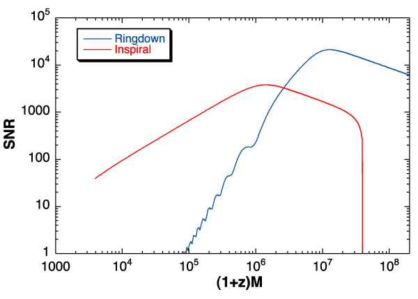
 , for the last
year of inspiral of an equal-mass MBH binary and for the ringdown after the merger of the system. The
method used to generate this figure follows that of [182], updated to use a modern LISA sensitivity
curve [277] with a low-frequency cutoff of
, for the last
year of inspiral of an equal-mass MBH binary and for the ringdown after the merger of the system. The
method used to generate this figure follows that of [182], updated to use a modern LISA sensitivity
curve [277] with a low-frequency cutoff of  . The redshift is set to
  , at which
the luminosity distance is
, at which
the luminosity distance is  using WMAP 7-year parameters [271].
 Reviews of the theory of quasi-normal modes can be found in Kokkotas and Schmidt [270], in
Nollert [337] and in Berti, Cardoso and Starinets [76], but we will briefly summarize the relevant results
here. At late times, the gravitational radiation from a perturbed black hole can be written as a sum
of exponentially-damped sinusoids. It is known that QNMs do not form a complete set in a
mathematical sense, but numerical results confirm that the late-time behavior is well described by
such an expansion [77]. The angular dependence can be decomposed into a sum of spheroidal
harmonics  of spin weight 2, which are labeled in analogy to standard spherical harmonics.
For each
of spin weight 2, which are labeled in analogy to standard spherical harmonics.
For each  , there are infinitely many resonant QNMs, which can be labeled in order of
decreasing damping time by a third parameter
, there are infinitely many resonant QNMs, which can be labeled in order of
decreasing damping time by a third parameter  . The waveform expansion takes the form

 ,
,  ,
,  , and
, and  are the frequency, damping time, amplitude, and initial phase of
the mode, and
are the frequency, damping time, amplitude, and initial phase of
the mode, and  is a complex number obtained by evaluating the spheroidal harmonics for the
particular orientation and mode frequency. The frequency and damping time,
is a complex number obtained by evaluating the spheroidal harmonics for the
particular orientation and mode frequency. The frequency and damping time,  and
and  , are
determined solely by the mass and frequency of the central black hole and are the key observables.
The damping time can also be considered as the reciprocal of the imaginary part of a complex
mode frequency, The amplitude and phase depend on the exact nature of the perturbation
that excited the QNMs, so they are less useful. One complication is that the mode numbers
that are excited [i.e., the
, are
determined solely by the mass and frequency of the central black hole and are the key observables.
The damping time can also be considered as the reciprocal of the imaginary part of a complex
mode frequency, The amplitude and phase depend on the exact nature of the perturbation
that excited the QNMs, so they are less useful. One complication is that the mode numbers
that are excited [i.e., the  parameters] are not known a priori. In the first analysis of
SNR from QNMs [182], it was assumed that only the
parameters] are not known a priori. In the first analysis of
SNR from QNMs [182], it was assumed that only the  ,
,  was excited, which
simplifies analysis of the observations. However, this simplifying assumption is not needed in
general.
was excited, which
simplifies analysis of the observations. However, this simplifying assumption is not needed in
general.
The use of QNMs as a probe of black-hole structure was first proposed by Dreyer et al. [155], who
coined the phrase “black-hole spectroscopy” for this technique. A measurement of  and
and
 for a single QNM will give several discrete solutions for the black-hole mass and spin,
corresponding to different choices for the mode numbers. A measurement of a second QNM
will give another discrete set of values, and in general these will not be the same as the first
set except for one combination, which are the true values [155]. This not only determines the
black-hole parameters, but provides a test that the central object is a Kerr black hole, since
the relationship between black-hole parameters and frequencies depends on that assumption.
If the object was something else, we would find no consistent combination of mass and spin
parameters to arise from the analysis. Dreyer et al. [155] considered a frequentist approach to
analyzing the QNM problem. The observable is a set of
for a single QNM will give several discrete solutions for the black-hole mass and spin,
corresponding to different choices for the mode numbers. A measurement of a second QNM
will give another discrete set of values, and in general these will not be the same as the first
set except for one combination, which are the true values [155]. This not only determines the
black-hole parameters, but provides a test that the central object is a Kerr black hole, since
the relationship between black-hole parameters and frequencies depends on that assumption.
If the object was something else, we would find no consistent combination of mass and spin
parameters to arise from the analysis. Dreyer et al. [155] considered a frequentist approach to
analyzing the QNM problem. The observable is a set of  complex QNM frequencies. We
denote a set of choices for the
complex QNM frequencies. We
denote a set of choices for the  modes to which the frequencies correspond by
  . Each
 defines a two-dimensional curve in the
  dimensional space, parameterized by
 . The probability distribution for the observed frequencies,
  , may be denoted by
 and can be used to define a confidence interval by determining the
  such that

 ,
,  and
and  . Using a toy model
for a non-black-hole source, and assuming that two QNMs were observed, drawn from four
possible excited modes, they estimated that, with a false alarm probability of 1%, the false
dismissal rate would be 60% if the SNR in the weakest mode was 10, falling to 10% at an SNR of
100. Assuming a reasonable amount of energy deposition into the QNMs, they estimated that
this would be satisfied by all LISA MBH merger sources, so the prospects for such tests are
good.
. Using a toy model
for a non-black-hole source, and assuming that two QNMs were observed, drawn from four
possible excited modes, they estimated that, with a false alarm probability of 1%, the false
dismissal rate would be 60% if the SNR in the weakest mode was 10, falling to 10% at an SNR of
100. Assuming a reasonable amount of energy deposition into the QNMs, they estimated that
this would be satisfied by all LISA MBH merger sources, so the prospects for such tests are
good.
Berti et al. [77] took a more detailed look at QNMs in general. They computed SNRs that improved on
those in [182] by using an up-to-date detector noise curve and including black-hole spin. For a
source of mass  at a distance of 3 Gpc, they found SNRs between 10
and
at a distance of 3 Gpc, they found SNRs between 10
and  for an excitation energy of 3% of the rest mass, and between 1 and 3000 for an
excitation energy of 0.1%. There is little dependence of the SNR on the central black-hole spin.
Putting the source at higher
for an excitation energy of 3% of the rest mass, and between 1 and 3000 for an
excitation energy of 0.1%. There is little dependence of the SNR on the central black-hole spin.
Putting the source at higher  shifts the sensitive range of masses in the usual way, but even at
redshift
shifts the sensitive range of masses in the usual way, but even at
redshift  the maximum SNR was found to be several hundred. Berti et al. [77] also
looked at parameter-estimation accuracy from observations of one QNM (with known mode
numbers) and found that LISA observations would measure the mass and spin to fractional
accuracies in the range
the maximum SNR was found to be several hundred. Berti et al. [77] also
looked at parameter-estimation accuracy from observations of one QNM (with known mode
numbers) and found that LISA observations would measure the mass and spin to fractional
accuracies in the range  for sources at
  and for the masses as quoted
above.
and for the masses as quoted
above.
Berti et al. [77] also performed a Fisher-matrix analysis of a two-mode problem, which accounted
for all correlations between the modes. They considered both “pseudo-orthonormal” modes
with different angular dependence ( or
or  ) and “overtones” – that is, modes
with the same angular dependence (
) and “overtones” – that is, modes
with the same angular dependence ( and
and  ). In both cases, the accuracy of
determination of the mass and spin was comparable to the results quoted for a single mode, although
the parameter space was simplified significantly to just five parameters:
). In both cases, the accuracy of
determination of the mass and spin was comparable to the results quoted for a single mode, although
the parameter space was simplified significantly to just five parameters:  ,
,  , two mode
amplitudes
, two mode
amplitudes  ,
,  , and a common initial phase
  . Berti et al. define two distinct QNMs
to have resolvable frequencies if the difference in these is larger than the error in both (and
similarly for the damping times). By recasting the two-mode model in terms of the two mode
frequencies and damping times rather than
. Berti et al. define two distinct QNMs
to have resolvable frequencies if the difference in these is larger than the error in both (and
similarly for the damping times). By recasting the two-mode model in terms of the two mode
frequencies and damping times rather than  and
and  , resolvability can be examined by looking
at the Fisher-matrix errors. Berti et al. [77] considered two cases (the resolvability of either
frequencies or damping times, and the resolvability of both), and they computed the source SNR
needed in each case. When the two modes are overtones, the SNR required to resolve “either”
was
, resolvability can be examined by looking
at the Fisher-matrix errors. Berti et al. [77] considered two cases (the resolvability of either
frequencies or damping times, and the resolvability of both), and they computed the source SNR
needed in each case. When the two modes are overtones, the SNR required to resolve “either”
was  100, the exact value depending on the black-hole spin and the (
 ,
, ) numbers
of the mode, but the SNR required to resolve “both” was
) numbers
of the mode, but the SNR required to resolve “both” was  1000. When the two modes
are “pseudo-orthonormal,” the SNR range to resolve “either” is
1000. When the two modes
are “pseudo-orthonormal,” the SNR range to resolve “either” is  a few if the modes differ
in
a few if the modes differ
in  , and
, and  a few tens if the modes have the same
  but differ in
  and the central
black-hole spin is
and the central
black-hole spin is  . There is a mode degeneracy, which means the SNR required blows
up when
. There is a mode degeneracy, which means the SNR required blows
up when  and
and  . The SNRs required to resolve “both” modes are in the range
100 – 10 000.
. The SNRs required to resolve “both” modes are in the range
100 – 10 000.
Berti et al. [77] conclude that even under pessimistic assumptions about the amount of energy radiated
in ringdown radiation, it should be possible to resolve one QNM and either the damping time or frequency
of a second QNM, provided that the first overtone radiates  of the total ringdown energy. This will
provide enough for a test of the no-hair property of the central object. A stronger test would come from
detecting frequencies and damping times for both QNMs, but this would require ringdown SNRs
of the total ringdown energy. This will
provide enough for a test of the no-hair property of the central object. A stronger test would come from
detecting frequencies and damping times for both QNMs, but this would require ringdown SNRs
 1000, which is rather unlikely. The main uncertainty in this analysis was in the excitation
coefficients for the various modes, but numerical relativity simulations have now provided some
information on the excitation of ringdown modes in a merger. Berti et al. revisited the QNM
problem in [72], using numerical relativity results presented in [74]. This paper revised downward
the SNR required to detect either the frequency or damping time of a second mode, which
is sufficient for a test of the no-hair theorem, to
1000, which is rather unlikely. The main uncertainty in this analysis was in the excitation
coefficients for the various modes, but numerical relativity simulations have now provided some
information on the excitation of ringdown modes in a merger. Berti et al. revisited the QNM
problem in [72], using numerical relativity results presented in [74]. This paper revised downward
the SNR required to detect either the frequency or damping time of a second mode, which
is sufficient for a test of the no-hair theorem, to  for any binary with mass ratio
greater than
for any binary with mass ratio
greater than  1.25. A significant fraction of LISA events should satisfy this criterion (see for
example [69]).
1.25. A significant fraction of LISA events should satisfy this criterion (see for
example [69]).
In [255], the authors used numerical-relativity simulations of nonspinning black-hole binaries, with a
variety of mass-ratios ranging from 1:1 to 1:11, to compute the amplitude to which several
different ringdown modes were excited, and hence an estimate of the SNR with which LISA
would be able to observe them. For all the mass ratios considered, the  mode was found
to radiate between 2% and 20% of the energy of the
mode was found
to radiate between 2% and 20% of the energy of the  mode, and for mass ratios more
unequal than 1:2 the
mode, and for mass ratios more
unequal than 1:2 the  also radiated more than 1% of the energy of the
  mode.
For sources at a redshift of
mode.
For sources at a redshift of  , they estimated a total ringdown SNR between 1000 and
20 000 for black-hole masses in the range
, they estimated a total ringdown SNR between 1000 and
20 000 for black-hole masses in the range  and mass ratios from 1:1 to 1:25, with
individual SNRs in the
and mass ratios from 1:1 to 1:25, with
individual SNRs in the  ,
,  , and
, and  modes between several hundred and 10 000.
The mode SNRs do not add in quadrature, but these SNRs more than meet the requirements
of [77] for LISA to be able to carry out black-hole spectroscopy. The SNRs realizable with
eLISA will be a few factors lower and the systems will tend to have lower masses, for which the
intrinsic SNRs are also smaller. Therefore constraints from eLISA will be weaker and it is possible
that eLISA will not be able to resolve sufficient separate modes, but this has not yet been
explored.
modes between several hundred and 10 000.
The mode SNRs do not add in quadrature, but these SNRs more than meet the requirements
of [77] for LISA to be able to carry out black-hole spectroscopy. The SNRs realizable with
eLISA will be a few factors lower and the systems will tend to have lower masses, for which the
intrinsic SNRs are also smaller. Therefore constraints from eLISA will be weaker and it is possible
that eLISA will not be able to resolve sufficient separate modes, but this has not yet been
explored.
In [210], Gossan et al. applied the results of [255] to explore the practicality of using QNM radiation to
test relativity. The authors considered mergers with mass ratios of 1:2 and constructed a waveform
model comprised of four ringdown modes. They used Bayesian methods and approached the
problem of testing relativity in two ways: (i) determining the parameters of each ringdown
mode separately and checking for consistency; (ii) comparing the Bayesian evidence of the GR
model to a non-GR model constructed by allowing for deviations of the mode parameters from
the GR predictions. The analysis was carried out for eLISA and for the Einstein Telescope,
the proposed third-generation ground-based detector. Gossan et al. showed that method (i)
could reveal inconsistencies of 1% in the QNM frequency for events of mass  at a
distance of 50 Gpc and inconsistencies of 10% for systems of mass
at a
distance of 50 Gpc and inconsistencies of 10% for systems of mass  at 6 Gpc. Better
constraints will come from systems at smaller distances and will therefore be observed with
higher SNR. Using method (ii), in the case of a signal from a
at 6 Gpc. Better
constraints will come from systems at smaller distances and will therefore be observed with
higher SNR. Using method (ii), in the case of a signal from a  black hole, 2%, 6%, and
10% deviations in the frequency of the dominant mode would be identifiable at distances of
approximately 1 Gpc, 5 Gpc, and 8 Gpc, respectively. Deviations of 2%, 6% and 10% in the
damping time of the dominant mode would only be detectable at distances of 200 Mpc, 700 Mpc,
and 1.2 Gpc, respectively. For a more massive system, of
black hole, 2%, 6%, and
10% deviations in the frequency of the dominant mode would be identifiable at distances of
approximately 1 Gpc, 5 Gpc, and 8 Gpc, respectively. Deviations of 2%, 6% and 10% in the
damping time of the dominant mode would only be detectable at distances of 200 Mpc, 700 Mpc,
and 1.2 Gpc, respectively. For a more massive system, of  , a 2% deviation in the
frequency/damping time of the dominant mode would be detectable out to 35/25 Gpc, but deviations
of 5% or more would be detectable at greater than 50 Gpc. Such massive systems are very
rare, however, and the choice of a 1:2 mass ratio means that the QNM radiation is stronger
than would be expected for typical eLISA events, which are likely to have larger mass ratios.
Therefore this study was limited in extent, but these preliminary results suggest that QNMs
could place interesting constraints on GR modifications for the strongest signals detected by
eLISA.
, a 2% deviation in the
frequency/damping time of the dominant mode would be detectable out to 35/25 Gpc, but deviations
of 5% or more would be detectable at greater than 50 Gpc. Such massive systems are very
rare, however, and the choice of a 1:2 mass ratio means that the QNM radiation is stronger
than would be expected for typical eLISA events, which are likely to have larger mass ratios.
Therefore this study was limited in extent, but these preliminary results suggest that QNMs
could place interesting constraints on GR modifications for the strongest signals detected by
eLISA.
Space-based QNM observations could be used directly to put constraints on alternative theories of gravity, but this will require a calculation of the QNMs in those alternative theories. It was shown in [501] that the equations governing black-hole perturbations in dynamical CS gravity were different from those in GR, with the consequence that the QNM spectrum would also be different. The authors did not compute QNMs, but QNM frequencies for non-spinning black holes in dynamical CS gravity were computed in [320]. The QNM spectrum was found to be different, due to the coupling of the black hole oscillations to the scalar field, but the detectability of these deviations by a gravitational-wave detector was not estimated. Therefore, it is not yet clear at what level ringdown radiation will be able to constrain the CS coupling parameter.
If a LISA-like observatory observes a MBH inspiral and does not detect QNM ringing from the merger
remnant where radiation would be expected, this might indicate a violation of the cosmic-censorship
hypothesis. QNM ringing arises as a result of GWs becoming trapped near the horizon of the black hole. If
a horizon was absent, for instance if a super-extremal ( ) Kerr metric was formed, we would not
expect to observe the QNM radiation. This would be evidence for the existence of a naked
singularity, and a counterexample to cosmic censorship, although not an indication of a problem with
GR.
) Kerr metric was formed, we would not
expect to observe the QNM radiation. This would be evidence for the existence of a naked
singularity, and a counterexample to cosmic censorship, although not an indication of a problem with
GR.
6.4 Prospects from gravitational-wave and other observations
Although there are still many open questions, current research clearly indicates that low-frequency GW detectors will be able to make strong statements about the structure of the massive compact objects in the centers of galaxies by observing EMRIs and by detecting ringdown radiation following supermassive black-hole mergers. At the very least, it will be possible to test that an observation is consistent with an inspiral into a Kerr black hole, and to state quantitatively how so large a deviation from Kerr could have been masked by instrumental noise. If a system differed significantly from Kerr, we would identify the deviation and should be able to quantify its nature. How well we would be able to distinguish between different types of deviation (e.g., external matter vs. a different multipole structure of the central object) is still not totally clear, but there are ongoing efforts in this direction.Another potential issue relates to modeling EMRIs. The tests of black-hole structure outlined in this section will rely on the detection of small differences between the observed GWs and the GWs expected in GR. This will of course rely on having reliable EMRI waveforms within GR. These waveforms can be computed using black-hole perturbation theory, by evaluating the gravitational self-force, but despite extensive work in this area the calculation of the self-force is not yet complete even at first order in the mass ratio. The first-order gravitational self-force has been computed for circular [48] and generic orbits in the Schwarzschild spacetime [49] and the scalar self-force is known for circular equatorial orbits in the Kerr spacetime [466]. Recently, the first self-force–driven inspirals have been computed, under an adiabatic approximation for the gravitational self-force [465], and self-consistently for the scalar self-force [151].9 EMRI models will require knowledge of the gravitational self-force for generic orbits in Kerr, which is still not available at first order. It has also been recognized that the radiative part of the second-order self-force will also be required to derive EMRI waveform phase to sufficient accuracy [238]. A formalism for the evaluation of the second-order self-force has been developed [366], but not yet implemented. Complete reviews of the current status of the self-force program can be found in [45, 362]. Additional complications in EMRI modeling arise from the need to accurately follow the transition of the inspiral through transient resonances [181]. Although many of these issues will have been resolved by the time data from a space-based gravitational-wave interferometer is available, they must be borne in mind in the interpretation of future results on tests of GR.
Low-frequency GW detectors will provide information on black-hole structure to a much higher precision
than can be achieved by other techniques. It has been suggested that observations of IMRIs with Advanced
LIGO will have some power to do similar tests [95]. This data will be available ten or more years prior to
any space-based experiment. However, IMRI-based tests will be much weaker, since many fewer cycles of
the GWs will be detected in a single observation due to the larger mass ratio ( );
furthermore, event rates are highly uncertain [302] and accurate modeling of IMRIs is far behind EMRI
modeling [239, 240]. An IMRI observation would be able to detect a deviation from Kerr of fractional order
unity in the quadrupole moment of a source [95], compared to the
);
furthermore, event rates are highly uncertain [302] and accurate modeling of IMRIs is far behind EMRI
modeling [239, 240]. An IMRI observation would be able to detect a deviation from Kerr of fractional order
unity in the quadrupole moment of a source [95], compared to the  fractional accuracies achievable
with LISA EMRIs [47].
fractional accuracies achievable
with LISA EMRIs [47].
Observations in the electromagnetic spectrum can also probe black-hole structure. Psaltis [371] provides
a thorough review of tests of strong-field gravity using electromagnetic observations. The most relevant tests
of black-hole structure are as follows.
- Horizon detection. X-ray interferometers (e.g., the Black Hole Imager) will soon have the
angular resolution to directly image the horizon of extragalactic black holes at distances of
 1 Mpc [371]. This is already almost possible with sub-mm/infrared observations. The
accretion flow for the Milky Way black hole, Sgr A*, can already be imaged directly down
to its innermost edge. However, interpretation of the observations is complicated by the need
to simultaneously constrain the disc properties. Observations at multiple wavelengths will be
required to fit out the disc and directly image the shadow of the black hole on the disc.
1 Mpc [371]. This is already almost possible with sub-mm/infrared observations. The
accretion flow for the Milky Way black hole, Sgr A*, can already be imaged directly down
to its innermost edge. However, interpretation of the observations is complicated by the need
to simultaneously constrain the disc properties. Observations at multiple wavelengths will be
required to fit out the disc and directly image the shadow of the black hole on the disc.
Evidence for the existence of horizons also comes from observations of quiescent X-ray binaries. An X-ray binary typically comprises a star filling its Roche lobe and transferring matter to a compact-object companion. That compact object can either be a neutron star or a black hole. If the object is a neutron star then most of the gravitational potential energy of the accreting matter has to be radiated away, but for black holes a significant amount of this energy can be advected through the black-hole horizon and is therefore not radiated to infinity [371
]. Among
systems in the same state of mass transfer, those containing neutron stars are expected to be
systematically more luminous than those containing black holes, as has been observed in our
galaxy.
Electromagnetic observations will really indicate the existence of a high-redshift surface in the system, and not necessarily an actual horizon. If a system contained a naked singularity with a high-redshift surface, but not a true event horizon, this would not be evident from the electromagnetic observations alone. By probing the multipole structure and verifying consistency with the no-hair theorem, LISA-like detectors will go much further.
- ISCO determination. The highest-temperature emission from a disc comes from the
innermost stable circular orbit (ISCO), and the flux at that temperature is proportional to the
ISCO radius squared. This allows the determination of the spin of the black hole. If the inferred
spin was found to exceed one, this might indicate failure in the black-hole model. Such spin
determinations have typical errors of
 10%, much greater than LISA’s expected errors of
 0.01% [46].
Indirect inference of the location of the inner edge of the accretion disc could also come from the interferometric observations mentioned above in the context of horizon detection. In [152] the authors use radio interferometry to resolve the base of the jet in the galaxy M87, finding it to be
 Schwarzschild radii. The jet-base radius is interpreted as being greater than
or equal to the radius of the innermost edge, so this system provides evidence for prograde
accretion onto a spinning black hole. Observations of jets in other nearby galaxies may follow
in the future, but the distance to which these structures could be resolved is quite small.
Schwarzschild radii. The jet-base radius is interpreted as being greater than
or equal to the radius of the innermost edge, so this system provides evidence for prograde
accretion onto a spinning black hole. Observations of jets in other nearby galaxies may follow
in the future, but the distance to which these structures could be resolved is quite small.
- Accretion-disc mapping. Particles in the accretion disc around a black hole move on circular
geodesics of the metric. If the orbits in the disc could be mapped, this would allow spacetime
mapping along the lines of Ryan’s theorem [387]. Two possible probes of accretion-disc
structure have been identified: quasi-periodic oscillation (QPO) pairs and iron K
 lines.
QPOs have been used to constrain possible values of black-hole masses and spins, but there are
uncertainties in the radius at which they originate, and in the resonance that gives rise to the
pairs of lines. Iron lines show broadening due to differential gravitational redshift and Doppler
shift at different points in the disc, but again their interpretation depends on unknown details
of the disc geometry. In principle, the time variability of an iron line after a single flare event
could constrain both the geometry and map the disc. Future observations with instruments
such as IXO/ATHENA will have the time-resolution to attempt this [371].
lines.
QPOs have been used to constrain possible values of black-hole masses and spins, but there are
uncertainties in the radius at which they originate, and in the resonance that gives rise to the
pairs of lines. Iron lines show broadening due to differential gravitational redshift and Doppler
shift at different points in the disc, but again their interpretation depends on unknown details
of the disc geometry. In principle, the time variability of an iron line after a single flare event
could constrain both the geometry and map the disc. Future observations with instruments
such as IXO/ATHENA will have the time-resolution to attempt this [371].
Electromagnetic observations are generally hampered by a lack of knowledge of the physics of the material that is generating the radiation. GW systems are, by contrast, very “clean” since the same theory describes the spacetime and the radiation generation. While there is some hope that future electromagnetic observations will perform crude spacetime mapping, LISA EMRI observations will improve any previous constraints by orders of magnitude.
 |
 |
 |
Living Rev. Relativity, 16 (2013), 7, doi:10.12942/lrr-2013-7, URL (accessed <date>): http://www.livingreviews.org/lrr-2013-7.
 This work is licensed under a Creative Commons License.
© The author(s), except where otherwise noted.
This work is licensed under a Creative Commons License.
© The author(s), except where otherwise noted.