5 Gravitational-Wave Tests of Gravitational Physics
Almost since its inception, GR was understood to possess propagating, undulatory solutions – GWs, described at leading order by the celebrated quadrupole formula [258]. It took several decades to establish firmly that these waves were real physical phenomena and not merely artifacts of gauge freedom.How would GW observations test the GR description of strong gravitational interactions, and possibly distinguish between GR and alternative theories? To answer this question we need to take a quick detour through GW data analysis. At least for foreseeable detectors, individual GW signals will typically be immersed in overwhelming noise, and therefore will need to be dug out with techniques akin to matched filtering [251], which by definition can only recover signals of shapes known in advance (the templates), or very similar signals. A matched-filtering search is set up by first selecting a parameterized template family (where the parameters are the source properties relevant to GW emission), and then filtering the detector data through discrete samplings of the family that cover the expected ranges of source parameters. The best-fitting templates correspond to the most likely parameter values, and by studying the quality of fits across parameter space it is possible to derive posterior probability densities for the parameters.
After a detection, the first-order question that we may ask is whether the best-fitting GR template is a satisfactory explanation for the measured data, or whether a large residual is left that cannot be explained as instrument noise, at least within our understanding of noise statistics and systematics. (Slightly more involved tests are also possible: for instance, we may divide measured signals in sections, estimate source parameters separately for each, and verify that they agree.) If a large residual is found, many hypotheses would be a priori more likely than a violation of GR: the fitting algorithm may have failed; another GW signal, possibly of unexpected origin, may be present in the data; the data may reflect a rare or poorly understood instrumental glitch; the GW source may be subject to astrophysical effects from nearby astrophysical objects, or even from intervening gravitational lenses.
Having ruled out such non-fundamental explanations, the only way to quantify the evidence for or
against GR is to consider it alongside an alternative model to describe the data. This alternative model
could be a phenomenological one (discussed below) or a self-consistent calculation within an
alternative theory of gravity. If the alternative theories under consideration include one or more
adjustable parameters that connect them to GR (such as  for Brans–Dicke theory, see
Section 2.1), and if those parameters can be propagated through the mathematics of source
modeling and GW generation, then GR template families can be enlarged to include them,
and the extra parameters can be estimated from GW observations. These extra parameters
may have a more phenomenological character, as would, for instance, a putative graviton mass
that would affect GW propagation, without finding direct justification in a specific theory.
Indeed, many of the “classic tests” discussed below (Section 5.1) fall within this class. To test
GR against “unconnected” theories without adjustable parameters, we would instead filter the
data through separate GR and alternative-theory template families, and decide which model
and theory are favored by the data using Bayesian model comparison, which we now describe
briefly.
for Brans–Dicke theory, see
Section 2.1), and if those parameters can be propagated through the mathematics of source
modeling and GW generation, then GR template families can be enlarged to include them,
and the extra parameters can be estimated from GW observations. These extra parameters
may have a more phenomenological character, as would, for instance, a putative graviton mass
that would affect GW propagation, without finding direct justification in a specific theory.
Indeed, many of the “classic tests” discussed below (Section 5.1) fall within this class. To test
GR against “unconnected” theories without adjustable parameters, we would instead filter the
data through separate GR and alternative-theory template families, and decide which model
and theory are favored by the data using Bayesian model comparison, which we now describe
briefly.
In complex data-analysis scenarios such as those encountered for GW detectors, the techniques of Bayesian inference [211, 414] are particularly useful for making assessments about the information content of data and for studying tests of gravitational theory, where the goal is to examine the hypothesis that the data might be described by some theory other than GR. In a traditional “frequentist” analysis of data, one computes the value of a statistic and then accepts or rejects a hypothesis about the data (e.g., that it contains a GW signal) based on whether or not the statistic exceeds a threshold. The threshold is set on the basis of a false-alarm rate, which is a statement about how the statistic would be distributed if the experiment was repeated many times. Evaluating the distribution of the statistic relies on a detailed and reliable understanding of the measurement process (noise, instrument response, astrophysical uncertainties, etc.). By contrast, Bayesian inference attempts to infer as much as possible about a particular set of data that has been observed, instead of making a statement about what would happen if the experiment were repeated.
Bayesian inference relies on the application of Bayes’ 1763 theorem: given the observed data  and a
parameterized model
and a
parameterized model  , the theorem relates the posterior probability of the parameters
given the data,
, the theorem relates the posterior probability of the parameters
given the data,  to the likelihood
  of observing the data
  given the
parameters
given the
parameters  , and the prior probability
  that the parameters would take that value:

 in the denominator is the evidence for the model
  . While
Eq. (35
. While
Eq. (35 ) follows trivially from the definition of conditional probability, its power comes from the idea of
updating the prior knowledge of a system given the results of observations. However, its practical
application is complicated by the necessity of attributing priors, and the correct evaluation of likelihoods
relies on the same detailed understanding of the statistical properties of the measurement noise as in the
frequentist case.
) follows trivially from the definition of conditional probability, its power comes from the idea of
updating the prior knowledge of a system given the results of observations. However, its practical
application is complicated by the necessity of attributing priors, and the correct evaluation of likelihoods
relies on the same detailed understanding of the statistical properties of the measurement noise as in the
frequentist case.
The evidence represents a measure of the consistency of the observed data with the model  , and can
be used to compare two models (e.g., the GR and modified-gravity descriptions of a GW-emitting system)
by evaluating the odds ratio for model 1 over model 2,
, and can
be used to compare two models (e.g., the GR and modified-gravity descriptions of a GW-emitting system)
by evaluating the odds ratio for model 1 over model 2,

 and
and  are the prior probabilities assigned for model 1 and 2 respectively. Either
model would be preferred if the odds ratio is sufficiently large/small, but the decision on which hypothesis
is best supported by the data is influenced by the choice of the priors, which will reflect the
analyst’s assessment of the relative correctness of the alternatives (see [451] for a discussion of this
point).
are the prior probabilities assigned for model 1 and 2 respectively. Either
model would be preferred if the odds ratio is sufficiently large/small, but the decision on which hypothesis
is best supported by the data is influenced by the choice of the priors, which will reflect the
analyst’s assessment of the relative correctness of the alternatives (see [451] for a discussion of this
point).
In the absence of well-defined alternative-theory foils, it may be desirable to proceed along the lines of the PPN formalism (Section 2.1) and immerse the GR predictions in expanded waveform families, designed to isolate differences in the resulting GW phenomenology (Section 5.2). Proposals to do so include schemes where the waveform-phasing post-Newtonian coefficients, which are normally deterministic functions of a smaller number of source parameters, are estimated individually from the data [28, 27]; the ambitiously-named parameterized post-Einstein (ppE) framework [497]; and the parameterization of Feynman diagrams for nonlinear graviton interactions [106]. In Section 5.3 we discuss ideas (so far rather sparse) to use the GWs from binary mergers-ringdowns to test GR.
We close these introductory comments by discussing two methodological caveats. First, GW observations are often characterized as “clean” tests of gravitational physics – whereby the “clean” emission of GWs from the bulk motion of matter (already emphasized above) is contrasted to “dirty” processes such as mass transfer, dynamical equation-of-state effects, magnetic fields, and so on. An even stronger notion of cleanness is important for the purpose of testing GR: for the best sources, the waveform signatures of alternative theories cannot be reproduced by changing the astrophysical parameters of the system – this orthogonality is quantified by the fitting factor between the GR and alternative-theory waveform families [451]. The degeneracy of the alternative-theory and source parameters would also lead to a “fundamental bias.” Fundamental bias arises from the assumption that the underlying theory in the analysis, generally taken to be GR, is the correct fundamental description for the physics being observed, which will impact the estimation of astrophysical quantities [497, 453].
Second, many of the results presented in this section rely on the Fisher-matrix formalism for
evaluating the expected parameter-estimation accuracy of GW observations [449]. As described
at the beginning of Section 4, the output of a GW detector is normally modeled as a linear
combination of a signal,  , and noise
  ,
,  . If the detector noise is assumed to
be Gaussian and stationary, the probability
. If the detector noise is assumed to
be Gaussian and stationary, the probability  is given by Eq. (30). The likelihood
 is just the probability that the noise takes the value
  , which is
![[ ( | ) ] p(d|⃗𝜃,M ) ∝ exp − 1- d − h(⃗𝜃)|d − h(⃗𝜃) , (37 ) 2 |](article298x.gif)
 is the inner product defined in Eq. (29). Writing
  and assuming
that we are close to the true parameters
and assuming
that we are close to the true parameters  , so that we can use the linear approximation
 (with
(with  ), we find that at quadratic order in
  where
is the Fisher information matrix. Thus, to leading order the shape of the likelihood in the vicinity of its
maximum is that of a multivariate Gaussian with covariance matrix
where
is the Fisher information matrix. Thus, to leading order the shape of the likelihood in the vicinity of its
maximum is that of a multivariate Gaussian with covariance matrix ![[ ( )( )] p(d |⃗𝜃,M ) ∝ exp − 1Γ jk Δ 𝜃j − (Γ − 1)jl(n|∂lh ) Δ 𝜃k − (Γ −1)km (n |∂mh ) , (38 ) 2](article305x.gif)

 (independent of
  ), and
the variance of the one-dimensional marginalized posterior probability density of parameter
), and
the variance of the one-dimensional marginalized posterior probability density of parameter  is
approximately
is
approximately  (no sum over
  ). This will be achieved in the limit of “high” signal-to-noise ratio
where the errors
). This will be achieved in the limit of “high” signal-to-noise ratio
where the errors  are small and the linear approximation is valid. The Fisher matrix arises also as the
Cramér–Rao lower bound on the variance of an unbiased estimator of the waveform parameters
are small and the linear approximation is valid. The Fisher matrix arises also as the
Cramér–Rao lower bound on the variance of an unbiased estimator of the waveform parameters  . A full
discussion of the various routes to the Fisher-matrix formula and its applications may be found
in [449].
. A full
discussion of the various routes to the Fisher-matrix formula and its applications may be found
in [449].
As emphasized by one of us [449], because the Fisher matrix is built with the first derivatives of waveforms with respect to source parameters, it can only “know” about the close neighborhood of the true source parameters. If the estimated errors take the waveform outside that neighborhood, then the formalism is simply inconsistent and unreliable. Higher SNRs reduce expected errors and therefore would generally make the formalism “safer,” but the meaning of “high” is problem dependent, depending on the number of parameters that need to be estimated, on their correlation, and on the strength of their effects on the waveforms.
In practice, only by carrying out a full computation of the posterior probability using, for example,
Monte Carlo methods will it be known if the Fisher matrix is providing a good guide to the
shape of the posterior. However, the Fisher matrix is generally much easier to compute than the
full posterior, so it is widely used as a guide to the precision with which parameters of the
model can be determined. In the context of testing GR, the Fisher matrix can be evaluated
for an expanded waveform model that includes non-GR-correction parameters, but at a set of
parameters that correspond to GR. The estimated error in the correction parameter,  , can
then be interpreted as the minimal size of a correction that would be detectable with a GW
observation.
, can
then be interpreted as the minimal size of a correction that would be detectable with a GW
observation.
5.1 The “classic tests” of general relativity with gravitational waves
As Will points out [469 , ch. 10], virtually any Lorentz-invariant metric theory of gravity must predict
gravitational radiation, but alternative theories will differ in its properties. Will identifies three main
properties that can be measured with GW detectors. These are the polarization, speed, and
emission multipolarity (monopole, dipole, quadrupole, etc.) of GWs in GR. In this paper, we
broaden the scope of the third to include changes to the loss of energy to GWs in inspiraling
systems.
, ch. 10], virtually any Lorentz-invariant metric theory of gravity must predict
gravitational radiation, but alternative theories will differ in its properties. Will identifies three main
properties that can be measured with GW detectors. These are the polarization, speed, and
emission multipolarity (monopole, dipole, quadrupole, etc.) of GWs in GR. In this paper, we
broaden the scope of the third to include changes to the loss of energy to GWs in inspiraling
systems.
In analogy to the three classic tests of GR (the perihelion of Mercury, deflection of light, and gravitational redshift) we like to refer to the verification that these properties have the predicted GR values, rather than the values predicted by alternative theories, as the “classic tests” of GR using GWs. Just as PPN tests probe weak-field, slow-motion dynamics, these tests can be seen as probing the weak-field far zone, where waves have propagated far from their sources. However, the multipolarity of GWs at emission and the energy that they carry away can be influenced by strong-field properties in the near zone where waves are generated.
5.1.1 Tests of gravitational-wave polarization
GR predicts the existence of two transverse quadrupolar polarization modes for GWs (also described as
“spin-2” and “tensor” using the language of group theory), usually labeled  and
and  . Alternative
metric theories of gravity predict as many as six polarizations [469] (three transverse and three
longitudinal), corresponding to the independent electric-type components of the Riemann curvature tensor,
. Alternative
metric theories of gravity predict as many as six polarizations [469] (three transverse and three
longitudinal), corresponding to the independent electric-type components of the Riemann curvature tensor,
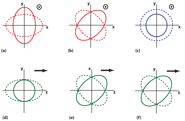
 . Schematically, these components are measured by GW detectors by monitoring the geodesic
deviation of nearby reference masses. The effect of different polarization modes is best illustrated by the
induced motion of a ring of test particles, as in Figure 4
. Schematically, these components are measured by GW detectors by monitoring the geodesic
deviation of nearby reference masses. The effect of different polarization modes is best illustrated by the
induced motion of a ring of test particles, as in Figure 4 . The response of a standard right-angle
interferometer to a scalar wave is maximal when the wave propagates along one arm; by contrast, tensor
modes elicit maximal response when the wave propagates in a direction perpendicular to the plane of the
detector.
. The response of a standard right-angle
interferometer to a scalar wave is maximal when the wave propagates along one arm; by contrast, tensor
modes elicit maximal response when the wave propagates in a direction perpendicular to the plane of the
detector.
 ].
].
Direct detection.
The use of GW polarization modes to test GR was first proposed in 1973 [160, 159]. The sensitivity of resonant and interferometric detectors, as well as Doppler-tracking and pulsar-timing measurements, to the extra modes was considered in several studies [343, 227, 412, 461, 292, 300, 324, 280, 331, 15, 118, 89, 225]. In the most general setting, the problem of disentangling the modes has eight unknowns – the time series for the six polarizations, plus two direction angles that affect the projection of the modes on the detector – but only six observables, corresponding to the components. Thus, the problem is indeterminate,
unless the source position is known from other observations (such as time-of-flight delays for a
long-baseline network of detectors), or unless we restrict GWs to transverse modes on theoretical
grounds.
Space-based observatories similar to LISA have either a single independent interferometric observable or
three (if laser links are maintained across all three arms). Each observable measures a different admixture of
polarizations. Thus, a detector with three active arms could in principle discriminate a non-GR polarization
mode if the direction to the source is known, or if it can be determined from the measured signal (by means
of the modulations produced by orbital motion, or by triangulation between the signals measured at the
three spacecraft).
components. Thus, the problem is indeterminate,
unless the source position is known from other observations (such as time-of-flight delays for a
long-baseline network of detectors), or unless we restrict GWs to transverse modes on theoretical
grounds.
Space-based observatories similar to LISA have either a single independent interferometric observable or
three (if laser links are maintained across all three arms). Each observable measures a different admixture of
polarizations. Thus, a detector with three active arms could in principle discriminate a non-GR polarization
mode if the direction to the source is known, or if it can be determined from the measured signal (by means
of the modulations produced by orbital motion, or by triangulation between the signals measured at the
three spacecraft).
The LISA sensitivity to alternative polarization modes was assessed in [440], using the full TDI
response (see Section 3.1). At frequencies larger than the inverse light-travel time along the arms,
LISA would be ten times more sensitive to scalar-longitudinal and vector modes [(d) to (f) in
Figure 4] than to tensor and scalar-transverse modes [(a) to (c) in Figure 4], because longitudinal
effects can accumulate as the lasers travel between the spacecraft. At lower frequencies, the
sensitivity to all modes is approximately the same. These results have not yet been used to work out
the constraints that LISA could place on specific alternative theories using different types of
sources.
In [26], a generic model for a system emitting dipole radiation in addition to quadrupole radiation was
constructed. The model was similar in structure to the ppE models which will be discussed in Section 5.2.2.
This model included both the dipolar component of the waveform, at the orbital frequency, and
modifications to the gravitational wave phasing of both the quadrupole and dipole waveform
components that arise from the additional energy lost into the dipole mode. In [26], the model was
used to determine the constraints on dipole radiation emission that would be possible using
ground-based GW detectors. Results for space-based detectors were included in a subsequent
review [31]. This demonstrated that eLISA would be able to place bounds on the parameter
 , that describes the observed amplitude of the dipole radiation relative to the quadrupole,
of
, that describes the observed amplitude of the dipole radiation relative to the quadrupole,
of  , and bounds on the parameter
  , which describes the amount of binary orbital
energy lost into the dipole radiation, of
, which describes the amount of binary orbital
energy lost into the dipole radiation, of  . The parameter
  affects the phase evolution
and so stronger bounds would be obtained for less massive systems, for which more waveform
cycles will be observed in band. These bounds are, in both cases, comparable to those from
observations with the Einstein Telescope, one order of magnitude better than those possible
with Advanced LIGO and one order of magnitude worse than what would be possible with
LISA.
affects the phase evolution
and so stronger bounds would be obtained for less massive systems, for which more waveform
cycles will be observed in band. These bounds are, in both cases, comparable to those from
observations with the Einstein Telescope, one order of magnitude better than those possible
with Advanced LIGO and one order of magnitude worse than what would be possible with
LISA.
Solar oscillations.
Finn [177] observed that solar oscillations with 5- to 10-minute periods produce
gravitational strains  at Earth, possibly within reach of space-based detectors. The detectors
would measure the sun’s dynamical gravitational field in the transition region where it is turning into
radiation. Finn showed that the field develops a significant phase shift relative to solar oscillations, which
depends on the GW polarizations, and which could distinguish between scalar, vector, tensor, and
scalar–tensor theories of gravity. The limit placed by such observations on the Brans–Dicke parameter
would be weaker than current bounds from solar-system tests; on the other hand, measuring incipient GWs
in the transition zone makes this a novel and possibly unique test. However, we note that Finn’s early
exploration [177] predates our full understanding of the design and parameters of LISA-like missions, which
are likely to be less sensitive to this signal. This problem was revisited in [140], in which the authors
assessed the sensitivity of LISA to the quadrupole (
at Earth, possibly within reach of space-based detectors. The detectors
would measure the sun’s dynamical gravitational field in the transition region where it is turning into
radiation. Finn showed that the field develops a significant phase shift relative to solar oscillations, which
depends on the GW polarizations, and which could distinguish between scalar, vector, tensor, and
scalar–tensor theories of gravity. The limit placed by such observations on the Brans–Dicke parameter
would be weaker than current bounds from solar-system tests; on the other hand, measuring incipient GWs
in the transition zone makes this a novel and possibly unique test. However, we note that Finn’s early
exploration [177] predates our full understanding of the design and parameters of LISA-like missions, which
are likely to be less sensitive to this signal. This problem was revisited in [140], in which the authors
assessed the sensitivity of LISA to the quadrupole ( ) low-order normal modes (
 ,
,  and
and
 -modes) of the sun. They estimated that the energy in these modes would have to exceed
 to allow a LISA detection, and that the required mode energy would be even higher for
eLISA.
to allow a LISA detection, and that the required mode energy would be even higher for
eLISA.
Galactic binaries.
Among the compact galactic binaries that would be detected by a LISA-like detector, several have orbital inclinations known from optical observations. For these systems we can compute the specific linear combination(s) of polarizations that would be appear in the data, which can then be checked for consistency. A single inconsistent binary may indicate an error in the determination of inclination or distance, but systematically inconsistent sources would hint at large non-tensor GW components. However, from general arguments the measurement accuracy for polarization amplitudes is (with SNR a
few tens at most for galactic binaries), so only very large corrections to GR would be detectable in this
way.
(with SNR a
few tens at most for galactic binaries), so only very large corrections to GR would be detectable in this
way.
5.1.2 Tests of gravitational-wave propagation
In GR, gravitational radiation propagates at the speed of light:  . The experimental validation of
this prediction can be posed as a bound on the graviton mass
. The experimental validation of
this prediction can be posed as a bound on the graviton mass  , which is exactly zero in GR
(see [59, 209] for a broader context). However, it may be advisable to consider
, which is exactly zero in GR
(see [59, 209] for a broader context). However, it may be advisable to consider  as a purely
phenomenological parameter, since certain massive-graviton theories do not recover GR predictions such as
light bending, as discussed in Section 2.2.5.
as a purely
phenomenological parameter, since certain massive-graviton theories do not recover GR predictions such as
light bending, as discussed in Section 2.2.5.
Weak-field measurements in the solar system already provide bounds on  on the basis of the
massive-graviton Yukawa correction to the Newtonian potential:
on the basis of the
massive-graviton Yukawa correction to the Newtonian potential:

 is the Compton wavelength of the graviton. The corresponding GW propagation speed
would be given by
with
is the Compton wavelength of the graviton. The corresponding GW propagation speed
would be given by
with 
 the frequency of radiation. The best solar-system tests provide the bound
  (or
(or  ) [435]. By contrast, binary-pulsar dynamics only provide a bound
 [178]. As we discuss in this section, observations of binary GWs with LISA-like
detectors could provide bounds competitive with these results, with the advantage of examining a rather
different sector of gravitational physics, wave propagation. Two distinct methods have been proposed for
this.
[178]. As we discuss in this section, observations of binary GWs with LISA-like
detectors could provide bounds competitive with these results, with the advantage of examining a rather
different sector of gravitational physics, wave propagation. Two distinct methods have been proposed for
this.
Comparing the phase of GW and EM signals.
This technique offers a direct comparison of the speed of GWs with the speed of a radiation assumed to be null (light itself). For the technique to work, sources must be observable in both light and GWs, and the astrophysical delays (if any) between the two signals must be well understood and modeled. The most prominent low-frequency sources for this purpose are compact galactic binaries. Let the difference between the arrival times of GWs and EM signals be where
 arises from propagation (the very effect we wish to measure), and
  from different
emission mechanisms or geometries. Here
from different
emission mechanisms or geometries. Here  is the redshift of the source, with
 the luminosity distance and
  the value of the Hubble parameter. In terms of
  ,
which we relate to
,
which we relate to 
 using the total relativistic energy,
where
using the total relativistic energy,
where 
 is the GW frequency.
The measurement of  has been considered repeatedly in the literature [279, 139, 128]. The main
difficulty lies with modeling the emission delay
has been considered repeatedly in the literature [279, 139, 128]. The main
difficulty lies with modeling the emission delay  : consider for instance AM CVn binaries,
where a low-mass helium donor has expanded to fill its Roche lobe and is spilling mass onto a
white-dwarf primary. The EM signal from these systems is greatly affected by the light emitted from
the overflow stream impacting the accretion disk, and the light curve oscillates as the system
orbits, alternately flashing the impact point toward and away from the observer. The times of
maximum emission can be taken as reference for the EM phase, but how are they related to GW
emission?
: consider for instance AM CVn binaries,
where a low-mass helium donor has expanded to fill its Roche lobe and is spilling mass onto a
white-dwarf primary. The EM signal from these systems is greatly affected by the light emitted from
the overflow stream impacting the accretion disk, and the light curve oscillates as the system
orbits, alternately flashing the impact point toward and away from the observer. The times of
maximum emission can be taken as reference for the EM phase, but how are they related to GW
emission?
To evaluate this  , one may observe the compact binary at two epochs, ideally at opposite points
across the Earth’s orbit [279, 139]. Under the assumption that
, one may observe the compact binary at two epochs, ideally at opposite points
across the Earth’s orbit [279, 139]. Under the assumption that  is constant, differencing the total
 measured at the two epochs leaves a measure of
  alone. However, the subtraction reduces
  to what can be accumulated across the diameter of the Earth’s orbit, rather than across the entire distance
to the binary. As a consequence, the strongest bound from known LISA verification binary would be
to what can be accumulated across the diameter of the Earth’s orbit, rather than across the entire distance
to the binary. As a consequence, the strongest bound from known LISA verification binary would be
 (
( ).
).
Alternatively, one may concentrate on eclipsing compact binaries, where the light curve varies due to the
mutual eclipses of the binary components, allowing the orientation geometry of the system to be precisely
determined as a function of time, and yielding an accurate measure of  . In this case the measured
 is accumulated over the entire distance to the source. Only one eclipsing binary that
would be observable with LISA-like detectors is currently known [230], but an analysis of their
statistically-expected population suggests that LISA would obtain a bound
is accumulated over the entire distance to the source. Only one eclipsing binary that
would be observable with LISA-like detectors is currently known [230], but an analysis of their
statistically-expected population suggests that LISA would obtain a bound  (
( ) [128].
The reader may question whether it is appropriate to compare gravitons to photons, when the current
bound on the putative mass of the photon is as high as  eV. However, the much higher
frequency of optical photons compared to low-frequency gravitons leads to
eV. However, the much higher
frequency of optical photons compared to low-frequency gravitons leads to  , much smaller
than
, much smaller
than  (for solar-system tests) [279], so a comparison based on speeds is indeed
appropriate.
(for solar-system tests) [279], so a comparison based on speeds is indeed
appropriate.
A related test using pulsar-timing observations would compare the GW-induced phase delays accumulated by photons traveling to Earth from different pulsars [281]: the delays depend on the graviton speed through a geometric factor that alters the expected Hellings–Downs correlation [228] that GWs will produce in the timing of pulsars located at different positions on the sky.
It might also be possible to observe simultaneous EM and GW signals from MBH mergers, using the approximate position of the source known from pre-merger GW observations to guide a follow-up campaign in the EM spectrum [267]. However, the nature of possible EM counterparts is extremely uncertain, so differences between the GW and EM phasing could be explained by uncertainties in the modeling of the EM signal. Therefore, it is unlikely that constraints from these systems will be competitive with galactic-binary constraints, or with the constraints from GW dispersion discussed in the following subsection.
Measuring the dispersion of gravitational-wave chirps.
The chirping signals emitted by inspiraling binaries contain a range of frequency components: if the graviton has mass, the components propagate at different speeds, again given by Eq. (44). This effect can be modeled in the templates used to search for binary
signals by including a  dependence in the waveform phasing [470]. In the frequency-domain
representation, the propagation effect appears as a “dephasing” term
dependence in the waveform phasing [470]. In the frequency-domain
representation, the propagation effect appears as a “dephasing” term  , where
 with
with  the binary chirp mass,
  the GW frequency,
  the source
distance, and
the source
distance, and  the source redshift. By comparison, the leading-order term in the post-Newtonian
expansion of the phasing is
the source redshift. By comparison, the leading-order term in the post-Newtonian
expansion of the phasing is  , while the
  correction contributes the same power of
orbital frequency as the “1PN” term.
For space-based detectors, the best chirp-dispersion bounds will come from massive–black-hole systems;
they improve slightly with the total binary mass and with better low-frequency (
correction contributes the same power of
orbital frequency as the “1PN” term.
For space-based detectors, the best chirp-dispersion bounds will come from massive–black-hole systems;
they improve slightly with the total binary mass and with better low-frequency ( )
sensitivity. However, the expected bounds depend strongly on which other physical effects (such as
spin-induced precessions, orbital eccentricity, higher waveform harmonics, the merger-ringdown phase) will
be relevant in the detected systems. As a result, a variety of predictions have appeared in the
literature [473, 70, 71, 32, 424, 485, 425, 259, 244]. Bounds as strong as
)
sensitivity. However, the expected bounds depend strongly on which other physical effects (such as
spin-induced precessions, orbital eccentricity, higher waveform harmonics, the merger-ringdown phase) will
be relevant in the detected systems. As a result, a variety of predictions have appeared in the
literature [473, 70, 71, 32, 424, 485, 425, 259, 244]. Bounds as strong as  a few
a few  seem possible, and would be strengthened by analyzing full catalogs of binary detections at
once [78].
seem possible, and would be strengthened by analyzing full catalogs of binary detections at
once [78].
Instead of the chirping signals from inspiraling binaries, Jones [253] proposes a test of the GW dispersion relation using the waves from eccentric galactic binaries, which are emitted at multiple harmonics of the orbital frequencies; if at least one galactic binary has sufficient eccentricity, Jones claims sensitivity comparable to the chirp-dephasing measurements. Mirshekari et al. [314] extend the graviton-mass formalism to more general modified-gravity theories that predict violations of Lorentz invariance and modified dispersion relations for GW modes, given by
both
 and
and  can be constrained together, given the
  corresponding to specific theories, by
inspiral-binary observations with ground and space-based detectors.
corresponding to specific theories, by
inspiral-binary observations with ground and space-based detectors.
Parity violations.
In GR parity is a conserved quantity, so left and right-circular polarized gravitational radiation propagates alike. Many attempts to formulate a quantum theory of gravity require the addition of a parity-violating Chern–Simons (CS) term to the Einstein–Hilbert action [14, 7, 363]: here
 is the Riemann tensor,
  is the Levi-Civita tensor density, and
  is a (possibly)
position-dependent function that describes the coupling of the CS field to spacetime. This correction creates
a difference in the propagation equations for the left- and right-circular GW polarizations, resulting in their
amplitude birefringence: one circularly-polarized state is amplified through propagation, while the other is
attenuated.
This effect is potentially observable with LISA-like detectors for MBH-binary inspirals at cosmological
distances [6] (see also [491]), where the amplitude birefringence generates an apparent precession of the
orbital plane of the binary. The CS correction accumulates with distance, and is larger for sources at higher
redshifts. Orbital-plane precession will also arise from general-relativistic spin–orbit coupling, but the
scaling of the precession with frequency is different, so the two effects can be distinguished, at least in
principle.
is a (possibly)
position-dependent function that describes the coupling of the CS field to spacetime. This correction creates
a difference in the propagation equations for the left- and right-circular GW polarizations, resulting in their
amplitude birefringence: one circularly-polarized state is amplified through propagation, while the other is
attenuated.
This effect is potentially observable with LISA-like detectors for MBH-binary inspirals at cosmological
distances [6] (see also [491]), where the amplitude birefringence generates an apparent precession of the
orbital plane of the binary. The CS correction accumulates with distance, and is larger for sources at higher
redshifts. Orbital-plane precession will also arise from general-relativistic spin–orbit coupling, but the
scaling of the precession with frequency is different, so the two effects can be distinguished, at least in
principle.
For an equal-mass binary with redshifted masses of  that is observed plane-on at a redshift
 , LISA could constrain the integrated CS contribution at the level of
  [6]. This is several
orders of magnitude better than solar-system experiments, which furthermore can only provide local
constraints. Thus, LISA-like detectors may provide some hints as to the very quantum nature of
gravity.
[6]. This is several
orders of magnitude better than solar-system experiments, which furthermore can only provide local
constraints. Thus, LISA-like detectors may provide some hints as to the very quantum nature of
gravity.
5.1.3 The quadrupole formula and loss of energy to gravitational waves
In theories that do not satisfy the strong equivalence principle, the internal gravitational binding energies of
bodies can create a difference between the inertial dipole moment (i.e., the linear momentum, which is
conserved) and the GW-generating gravitational dipole moment. Thus, alternative theories of gravity
generally admit dipole radiation, but it is forbidden in GR, where the two moments are identical. Dipole
radiation would be given at leading order by [471]

 are the positions of the binary components,
  their relative velocity,
  and
and  are
their inertial and gravitational masses respectively,
are
their inertial and gravitational masses respectively,  is the inertial reduced mass, and
  is the
luminosity distance to the observer.
is the
luminosity distance to the observer.
For relativistic objects such as neutron stars (NS), the gravitational binding energy can be considerable
and so can be the resulting loss of energy to dipolar GWs. Indeed, the experimental result that the orbital
decay of the binary pulsar PSR1913+16 [293] adhered closely to GR’s quadrupole-formula prediction was
sufficient to definitely falsify GR alternatives such as bimetric and “stratified” theories [469]. (Amusingly,
certain theories even predict that dipole radiation carries away negative energy from a binary [469].) Thus
it is factually correct to state that the indirect detection of GWs has already provided a strong test of
GR.
By contrast, the binary pulsar could not falsify scalar-tensor theories in this way, because these are
“close” to GR. For instance, although dipole radiation is predicted by Brans–Dicke theory and changes the
progression of orbital decay, the coupling parameter  can be adjusted to approximate GR
results to any desired accuracy. GR is reproduced for
can be adjusted to approximate GR
results to any desired accuracy. GR is reproduced for  , so experimental bounds on
Brans–Dicke are lower bounds. The Hulse–Taylor binary pulsar does provide a bound on
, so experimental bounds on
Brans–Dicke are lower bounds. The Hulse–Taylor binary pulsar does provide a bound on  , but
one that is not competitive with solar-system tests, among which the best comes from the
Doppler tracking of the Cassini spacecraft, which sets
, but
one that is not competitive with solar-system tests, among which the best comes from the
Doppler tracking of the Cassini spacecraft, which sets  [471, 81]. However, other
binary systems containing pulsars are known that provide constraints, which are competitive
with solar-system constraints. The best constraints on scalar-tensor gravity (and also TeVeS
gravity) come from the pulsar–white-dwarf binary J1738+0333 [186], which provides the limit
[471, 81]. However, other
binary systems containing pulsars are known that provide constraints, which are competitive
with solar-system constraints. The best constraints on scalar-tensor gravity (and also TeVeS
gravity) come from the pulsar–white-dwarf binary J1738+0333 [186], which provides the limit
 .
.
LISA-like detectors can constrain  by looking for dipole-radiation–induced modifications in the
GW phasing of binary inspirals (monopole radiation is also present, but suppressed relative to
the dipole), as long as at least one of the binary components is not a black hole: because of
the no-hair theorem, black holes cannot sustain the scalar field that would lead to a differing
by looking for dipole-radiation–induced modifications in the
GW phasing of binary inspirals (monopole radiation is also present, but suppressed relative to
the dipole), as long as at least one of the binary components is not a black hole: because of
the no-hair theorem, black holes cannot sustain the scalar field that would lead to a differing
 and
and  (as was recently confirmed in full numerical-relativity simulations [226]). This
restriction can be circumvented by having non-asymptotically flat boundary conditions for
the black hole [237]. If the scalar field is slowly varying far from the black hole (either as a
function of time or space) then it can support a scalar field. This scenario was investigated
numerically in [75], which found that accelerated single black holes and black-hole binaries
would emit scalar radiation, in the latter case at twice the orbital frequency. If the asymptotic
scalar-field gradient that supports the black-hole scalar hair is cosmological in origin, this effect
will be negligible, but the possibility does exist in general. Except for these considerations,
the canonical source for detecting this effect is the inspiral of a neutron star into a relatively
low-mass central black hole, although the number of detections of such systems is likely to be very
low [192].
(as was recently confirmed in full numerical-relativity simulations [226]). This
restriction can be circumvented by having non-asymptotically flat boundary conditions for
the black hole [237]. If the scalar field is slowly varying far from the black hole (either as a
function of time or space) then it can support a scalar field. This scenario was investigated
numerically in [75], which found that accelerated single black holes and black-hole binaries
would emit scalar radiation, in the latter case at twice the orbital frequency. If the asymptotic
scalar-field gradient that supports the black-hole scalar hair is cosmological in origin, this effect
will be negligible, but the possibility does exist in general. Except for these considerations,
the canonical source for detecting this effect is the inspiral of a neutron star into a relatively
low-mass central black hole, although the number of detections of such systems is likely to be very
low [192].
Early studies [397, 473], based on simplified models of the waveforms and of the LISA sensitivity,
estimated that for a  neutron star inspiraling into a MBH, at fixed SNR = 10, the
  bounds
would scale as
bounds
would scale as

 (the “sensitivity”) is a measure of the difference between the neutron-star and MBH
self-gravitational binding energies per unit rest mass;
(the “sensitivity”) is a measure of the difference between the neutron-star and MBH
self-gravitational binding energies per unit rest mass;  is the dipole contribution to the GW phasing;
 is the time of observation; and
  is the MBH mass. However, this estimate is reduced by a factor of
ten or more when more realistic waveforms are considered that include spin couplings [70, 71], spin-induced
orbital precession and eccentricity [485]. Bounds can also be derived for a massive-scalar variant of
Brans–Dicke theory [79], and are of order
(where
is the MBH mass. However, this estimate is reduced by a factor of
ten or more when more realistic waveforms are considered that include spin couplings [70, 71], spin-induced
orbital precession and eccentricity [485]. Bounds can also be derived for a massive-scalar variant of
Brans–Dicke theory [79], and are of order
(where 
 is the mass of the scalar and
  the detection SNR) for the intermediate–mass-ratio inspiral
of a NS into a black hole with mass
the detection SNR) for the intermediate–mass-ratio inspiral
of a NS into a black hole with mass  .
.
These results were obtained using only the leading order correction from the scalar radiation. In [495] the authors extended this calculation to all post-Newtonian orders, but in the extreme-mass-ratio limit by using the Teukolsky formalism. The conclusion, that constraints on massless scalar-tensor theories from GW observations will, in general, be weaker than those from solar-system observations, was unchanged. The reason is that scalar-tensor theories are weak-field (infrared) corrections to GR and are therefore largest in the weak field, so the leading order correction captures the majority of the effect. Massive scalar-tensor theories were also considered in [110, 495]. In those theories, the primary observable consequence is the possible existence of “floating orbits” at which the scalar flux experiences a condition where GWs scatter off the central, massive body, emerging with more energy (extracted from the spin of the central body). The waves transfer that energy to the small orbiting body, increasing its orbital energy. This “super-radiant resonance” temporarily balances the GW flux. The transition of an EMRI through such a floating orbit is many orders of magnitude slower than the normal EMRI inspiral and can last more than a Hubble time. If an EMRI consistent with GR is observed it means that the EMRI not only did not pass through such a floating orbit during the timescale of the observation but could not have encountered one prior to the observation since it would not then have reached the millihertz band. Therefore, an observation of a single EMRI can constrain the massive scalar-tensor parameter space to many orders of magnitude greater precision than current solar-system observations.
Other modifications to the inspiral phasing.
A number of other suggestions have been made for low-frequency GW tests of GR that do not quite fit a “modified energy-loss” description. For instance, dynamical Chern–Simons theory introduces nonlinear modifications in the binary binding energy and dissipative corrections at the same PN order [426, 483] that could be observed in the late inspiral,
constraining the characteristic Chern–Simons length scale  to
to  [487], comparable to
current solar-system constraints [13] (advanced ground-based detectors could do even better, placing
bounds of
[487], comparable to
current solar-system constraints [13] (advanced ground-based detectors could do even better, placing
bounds of  ).
Corrections to the inspiral phasing will also arise if the spacetime outside the central object is not
described by the Kerr metric or if additional energy is lost into scalar or other forms of radiation. This has
been considered for various alternative theories of gravity; we discuss these results in detail in
Section 6.2.6.
).
Corrections to the inspiral phasing will also arise if the spacetime outside the central object is not
described by the Kerr metric or if additional energy is lost into scalar or other forms of radiation. This has
been considered for various alternative theories of gravity; we discuss these results in detail in
Section 6.2.6.
GW tails, which are due to the propagation of gravitational radiation on the curved background of the
emitting binary, appear at a relative 1.5PN order ( ) beyond the leading-order quadrupole radiation,
and their observation would test the nonlinear nature of GR [88]. (This would be a null test of GR, since
tails are included in the “standard” post-Newtonian inspiral phasing; see also the PN-coefficient tests
discussed in Section 5.2.1.
) beyond the leading-order quadrupole radiation,
and their observation would test the nonlinear nature of GR [88]. (This would be a null test of GR, since
tails are included in the “standard” post-Newtonian inspiral phasing; see also the PN-coefficient tests
discussed in Section 5.2.1.
Promoting Newton’s constant,  , to a function of time modifies both a binary’s binding energy and
GW luminosity, and therefore its phasing. A three-year observation of a
, to a function of time modifies both a binary’s binding energy and
GW luminosity, and therefore its phasing. A three-year observation of a  inspiral would
constrain
inspiral would
constrain  to
to  [498]. The infinite Randall–Sundrum braneworld model [373] may
predict an enormous increase in the Hawking radiation emitted by black holes [164, 436]. The resulting
progressive mass loss may be observed as an outspiral effect in the quasi-monochromatic radiation of
galactic black-hole binaries, as a correction to the inspiral phasing of a black-hole binary [484] and it would
also affect the rate of EMRI events [306, 484]. The constraints on the size of extra dimensions coming from
observations with LISA will, in general, be worse than those derivable from tabletop experiments. However,
DECIGO observations of BH–NS binary mergers would be able to place a constraint about
ten times better than tabletop experiments, assuming a detection rate of
[498]. The infinite Randall–Sundrum braneworld model [373] may
predict an enormous increase in the Hawking radiation emitted by black holes [164, 436]. The resulting
progressive mass loss may be observed as an outspiral effect in the quasi-monochromatic radiation of
galactic black-hole binaries, as a correction to the inspiral phasing of a black-hole binary [484] and it would
also affect the rate of EMRI events [306, 484]. The constraints on the size of extra dimensions coming from
observations with LISA will, in general, be worse than those derivable from tabletop experiments. However,
DECIGO observations of BH–NS binary mergers would be able to place a constraint about
ten times better than tabletop experiments, assuming a detection rate of  binaries per
year [484].
binaries per
year [484].
5.2 Tests of general relativity with phenomenological inspiral template families
As discussed above, quantitative tests of GR against modified theories of gravity evaluate how well the
measured signals are fit by alternative waveform families, or (more commonly) by waveform families that
extend GR predictions by including one or more modified-gravity parameters, such as  for
Brans–Dicke theory. To set up these tests we need to work within the alternative theory to derive
sufficiently accurate descriptions of source dynamics, GW emission, and GW propagation. An alternative
approach is to operate directly at the level of the waveforms by introducing phenomenological
corrections to GR predictions: for instance, by modifying specific coefficients, or by adding extra
terms.
for
Brans–Dicke theory. To set up these tests we need to work within the alternative theory to derive
sufficiently accurate descriptions of source dynamics, GW emission, and GW propagation. An alternative
approach is to operate directly at the level of the waveforms by introducing phenomenological
corrections to GR predictions: for instance, by modifying specific coefficients, or by adding extra
terms.
This section discusses the first attempts to do so. So far these have concentrated on post-Newtonian waveforms [84] for circular, adiabatic inspirals, as described by the stationary-phase approximation in the frequency domain:
where![[ π ] &tidle;h (f) = Af −7∕6exp iΨ(f ) + i- , (50 ) 4](article429x.gif)
 is the GW frequency;
  is the GW amplitude, given by geometrical projection factors
 (with
(with  the chirp mass and
  the luminosity distance); and
for simplicity we omit the nontrivial response of space-based detectors, as well as the PN amplitude
corrections. The phasing
the luminosity distance); and
for simplicity we omit the nontrivial response of space-based detectors, as well as the PN amplitude
corrections. The phasing  is expanded as
For binaries with negligible component spins, the post-Newtonian phasing coefficients
is expanded as
For binaries with negligible component spins, the post-Newtonian phasing coefficients ![[ ] ∑ log (k−5)∕3 Ψ (f) = 2πf tc + Φc + ψk + ψk log f f . (51 ) k∈ℤ](article437x.gif)
 are currently
known up to
are currently
known up to  (3.5 PN order), and in GR they are all functions of the two masses
  and
and  alone (although
  , and
, and  is completely degenerate with
  , so it is usually
omitted) [86, 87, 85, 30].
, so it is usually
omitted) [86, 87, 85, 30].
5.2.1 Modifying the PN phasing coefficients
Arun et al. [28] propose a test of GR based on estimating all the  simultaneously
from the measured waveform as if they were free parameters, in analogy to the
post-Keplerian formalism [293, Section 4.5]. The value and error estimated for
each4
simultaneously
from the measured waveform as if they were free parameters, in analogy to the
post-Keplerian formalism [293, Section 4.5]. The value and error estimated for
each4
 , together with its PN functional form as a function of
  and
and  , determines a region in the
 –
– plane. If GR is correct, all the regions must intersect near the true masses, as shown in
Figure 5. The extent of the intersection provides a measure of how precisely GR is verified by a GW
observation. A Fisher-matrix analysis [28] suggests that, for systems at the optimistic distance of 3 Gpc,
LISA could measure
plane. If GR is correct, all the regions must intersect near the true masses, as shown in
Figure 5. The extent of the intersection provides a measure of how precisely GR is verified by a GW
observation. A Fisher-matrix analysis [28] suggests that, for systems at the optimistic distance of 3 Gpc,
LISA could measure  to
to  0.1% and
  and
and  to 10%, but that the fractional error on
higher-order terms would be at best
to 10%, but that the fractional error on
higher-order terms would be at best  1.
1.
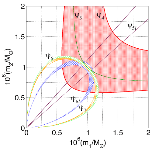
 of Eq. (
 –
– plane, which must intersect near true mass values if GR is correct.
Image reproduced by permission from
plane, which must intersect near true mass values if GR is correct.
Image reproduced by permission from However, this setup may understate the power of this kind of test, since most of the estimation
uncertainty in the  arises from their mutual degeneracy – that is, from the fact that it is possible to
vary the value of a subset of
arises from their mutual degeneracy – that is, from the fact that it is possible to
vary the value of a subset of  without appreciably modifying the waveform. This degeneracy
should not impact the degree to which the data is deemed consistent with GR. In a follow-up
paper [27], Arun et al. propose a revised test whereby the masses are determined from
without appreciably modifying the waveform. This degeneracy
should not impact the degree to which the data is deemed consistent with GR. In a follow-up
paper [27], Arun et al. propose a revised test whereby the masses are determined from  and
and  , while the other
  (as well as
  and
and  ) are individually estimated and
checked for consistency with GR. In this case, even for sources at
) are individually estimated and
checked for consistency with GR. In this case, even for sources at  (
( 7 Gpc), all the
parameters can be constrained to 1% (a few % for
7 Gpc), all the
parameters can be constrained to 1% (a few % for  , 0.1% for
  ), at least for favorable
mass combinations. Performing parameter estimation for the eigenvectors of the
), at least for favorable
mass combinations. Performing parameter estimation for the eigenvectors of the  Fisher
matrix [342] indicates which combinations of coefficients can be tested more accurately for GR
violations.
Fisher
matrix [342] indicates which combinations of coefficients can be tested more accurately for GR
violations.
However, it is not clear what significance with regards to testing GR should be ascribed to the accuracy
of measuring the  , since we do not know at what level we could expect deviations to appear. By
contrast, if we were to find that, say, the
, since we do not know at what level we could expect deviations to appear. By
contrast, if we were to find that, say, the  –
– regions in the
  –
– plane do not intersect, we
could make the statistically-meaningful statement that GR appears to be violated at the
plane do not intersect, we
could make the statistically-meaningful statement that GR appears to be violated at the  –
– level.
Del Pozzo et al. [148] and Li et al. [284, 285] propose a more satisfying formulation for these tests,
based on Bayesian model selection [211], which compares the Bayesian evidence, given the observed data,
for the pure-GR scenario against the alternative-gravity scenarios in which one or more of the  are
modified. The issue of significance discussed above reappears in this context as the inherent
arbitrariness in choosing prior probabilities for the
are
modified. The issue of significance discussed above reappears in this context as the inherent
arbitrariness in choosing prior probabilities for the  , but Del Pozzo et al. argue that this
does not affect the efficacy of the model-comparison test in detecting GR violations. (For a
comprehensive discussion of model selection in the context of GW detection, rather than GR tests, see
also [456, 457, 291]. For more recent applications of this formalism to ground-based detectors,
see [315].)
, but Del Pozzo et al. argue that this
does not affect the efficacy of the model-comparison test in detecting GR violations. (For a
comprehensive discussion of model selection in the context of GW detection, rather than GR tests, see
also [456, 457, 291]. For more recent applications of this formalism to ground-based detectors,
see [315].)
5.2.2 The parameterized post-Einstein framework
In [497], Yunes and Pretorius propose a similar but more general approach, labeling it the “parameterized post-Einsteinian” (ppE) framework. For adiabatic inspirals, they propose enhancing the stationary-phase inspiral signal with extra powers of GW frequency:
where![&tidle;hppE(f) = &tidle;hGR (f) × (1 + α (πℳf )a)exp [iβ(πℳf )b], (52 )](article484x.gif)
 is given in Eqs. (50) and (51). While the initial suggestion in [497] is to consider
 , there are analytical arguments why
  and
and  should be restricted to values
  and
and
 , with
  [120], which reproduces Arun’s PN-coefficient scheme for
  .
Nevertheless, this representation can reproduce the leading-order effects of several alternative theories of
gravity (see Table 2).
)]. For GR
.
Nevertheless, this representation can reproduce the leading-order effects of several alternative theories of
gravity (see Table 2).
)]. For GR  . This table is copied from [134], except for the two entries labeled
with an asterisk. The quadratic curvature ppE exponent given in [134] was
. This table is copied from [134], except for the two entries labeled
with an asterisk. The quadratic curvature ppE exponent given in [134] was  , coming
from the conservative dynamics. However, it was shown in [483] that the dissipative correction is
larger, giving the value
, coming
from the conservative dynamics. However, it was shown in [483] that the dissipative correction is
larger, giving the value  quoted above. The dynamical Chern–Simons ppE exponent given
in [134] was
quoted above. The dynamical Chern–Simons ppE exponent given
in [134] was  , which was derived using the slow-rotation metric accurate to linear order
in the spin [496]. At quadratic order in the spin [488], the corrections to both conservative and
dissipative dynamics occur at lower post-Newtonian order, giving
, which was derived using the slow-rotation metric accurate to linear order
in the spin [496]. At quadratic order in the spin [488], the corrections to both conservative and
dissipative dynamics occur at lower post-Newtonian order, giving  [487].
 |
 |
 |
 |
|
| Brans–Dicke | – | 0 | –7/3 |  |
| parity violating | 1 |  |
0 | – |
variable  |
–8/3 |  |
–13/3 |  |
| massive graviton | – | 0 | –1 |  |
| quadratic curvature | – | 0 | –7/3* |  |
| extra dimensions | – | 0 | –13/3 |  |
| dynamical Chern–Simons | +3 |  |
+1/3 |  |
In [497], Yunes and Pretorius are motivated by the possibility of detecting GR violations, but also by
the “fundamental bias” that would be incurred in estimating GW-source parameters using GR waveforms
when modified GR is instead correct. In [134], Cornish et al. reformulate the detection of GR violations
described by ppE as a Bayesian model-selection problem, similar to the PN-coefficient tests
discussed in Section 5.2.1. Figure 6 shows the  bounds, for various fixed
  , that could
be set with LISA observations of
, that could
be set with LISA observations of  binary inspirals at
  and 3. For
  corresponding to modifications in higher-order PN terms (which require strong-field, nonlinear
gravity conditions to become evident), the bounds provided by LISA-like detectors become more
competitive with respect to solar-system and binary-pulsar results (where weak-field conditions
prevail).
corresponding to modifications in higher-order PN terms (which require strong-field, nonlinear
gravity conditions to become evident), the bounds provided by LISA-like detectors become more
competitive with respect to solar-system and binary-pulsar results (where weak-field conditions
prevail).
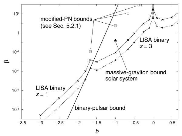
 massive–black-hole inspirals at
  and
and  . The figure also
includes the
. The figure also
includes the  bounds derived from pulsar PSR J0737–3039 [492], the solar-system bound on
the graviton mass [435], and PN-coefficient bounds derived as described Section 5.2.1. The spike
at
bounds derived from pulsar PSR J0737–3039 [492], the solar-system bound on
the graviton mass [435], and PN-coefficient bounds derived as described Section 5.2.1. The spike
at  corresponds to the degeneracy between the ppE correction and the initial GW-phase
parameter. (Adapted from [134].)
corresponds to the degeneracy between the ppE correction and the initial GW-phase
parameter. (Adapted from [134].) A ppE-like model including dipole radiation in addition to quadrupole radiation but no other
modifications to the waveform phasing was described in [26] and was discussed in Section 5.1.1
above. The full ppE framework was extended to include all additional polarization states and
higher waveform harmonics in [120]. The final form was motivated by considering Brans–Dicke
theory, Lightman–Lee theory and Rosen’s theory. In the most general form, Eq. 52 is modified to
![&tidle;ppE &tidle; GR [ b] h (f) = h (f) × exp iβ (πℳf ) + (α+F+ + α×F × + αbFb + αLFL + αsnFsn + αseFse) [ (2) ] × (π ℳf )aexp − iΨ GR + iβ (πℳf )b + (α+F+ + α×F × + αbFb + αLFL + αsnFsn + αs[eFse) ] × (2 πℳf )cη15 exp − iΨ (1) + iδ(2πℳf )d , (53 ) GR](article523x.gif)
 is the GR phase of the
  th waveform harmonic,
  is the
symmetric mass ratio, and
is the
symmetric mass ratio, and  is the detector response to a GW in polarization mode
  . The ppE
parameters are
. The ppE
parameters are  .
.
The authors of [120] considered two further variants of this scheme. One variant restricted the coefficients in the expansion so that they were not all independent, but were related to one another via energy conservation. The second variant included this interdependence of the parameters, and also accounted for modified propagation effects by introducing additional “phase-difference” parameters into the second and third terms. As yet, this fully extended ppE scheme has not been used to explore the constraints that will be possible with space-based detectors.
An analysis using a waveform model with higher harmonics and spin precession, but not alternative
polarization states, was carried out in [244]. Its authors considered modifications to a subset of the phase
and amplitude parameters only, which corresponded to certain post-Newtonian orders and
could therefore also be interpreted in terms of modifications to the pN phase coefficients as
discussed in Section 5.2.1. The estimated bounds derived using this more complete waveform model
were typically one to two orders of magnitude better than previous estimates for high-mass
systems, but basically the same for low-mass systems. This is unsurprising, since the effects of
spin-precession and higher harmonics will only be important late in the inspiral. High-mass systems
generate lower frequency GWs and are therefore only observable for the final stages of inspiral,
merger and plunge. Therefore, late-time corrections are proportionally more important for those
systems. For high-mass systems, the authors of [244] estimated that LISA would be able to
measure deviations in the phasing parameters to a precision  for
for
 respectively, where
  denotes the post-Newtonian order, with
  the coefficient
of
the coefficient
of  in the waveform phase. Using the same model, they also estimated that LISA could
place a bound of
in the waveform phase. Using the same model, they also estimated that LISA could
place a bound of  on the graviton Compton wavelength when allowing for
correlations between the different phase-modification parameters
on the graviton Compton wavelength when allowing for
correlations between the different phase-modification parameters  . This was discussed in
Section 5.1.2.
. This was discussed in
Section 5.1.2.
An extension of the ppE framework to EMRI systems requires a model in which orbits can be both
eccentric and inclined. To develop this, Vigeland et al. [458] derive a set of near-Kerr spacetime metrics
that satisfy a set of conditions, including the existence of a Carter-constant–like third integral of the
motion, as well as asymptotic flatness. The solutions, which were previously found in [65],
are restricted to a physically interesting subset by setting to zero any metric coefficients not
required to reproduce known black-hole solutions in modified gravity, and by applying the peeling
theorem (i.e., by requiring that the mass and spin of the black hole not be renormalized by the
perturbation).
The existence of a third integral is not a requirement for black-hole solutions, but in general its absence allows ergodic behavior in the orbits. This is discussed as a potential observable signature for deviations from GR in Section 6.2.5. However, data-analysis pipelines designed for GR waveforms may be insensitive to such qualitatively different systems. Therefore the existence of a third integral is a practical assumption for interpretation once a GR-like EMRI has been observed.
In [201], Gair and Yunes construct gravitational waveforms for EMRIs occurring in the metrics
of [458], based on the analytic kludge model constructed for GR EMRIs [46]. The waveforms
provide a ppE-like model for EMRIs that can be used in the same way as the circular ppE
framework. Parameter-estimation results with these ppE–EMRI models have not yet appeared in the
literature.
5.2.3 Other approaches
In [451], Vallisneri provides a unified model-comparison performance analysis of all modified-GR tests that is valid for sufficiently-loud signals, and that yields the detection SNR required for a statistically-significant detection of GR violations as a simple function of the fitting factor FF between the GR and modified-GR waveform families. The FF measures the extent to which one can reabsorb modified-GR effects by varying standard-GR parameters from their true values. Vallisneri’s analysis is valid in the limit of large SNR, and may not be applicable to all realistic scenarios with finite SNRs.
An alternative to modifying frequency-domain inspiral waveforms is offered by Cannella et
al. [106, 105]. They propose tests based on the effective-field-theory approach to binary dynamics [208],
which expands the Hilbert+point-mass action as a set of Feynman diagrams. In this framework, GR
corrections can be introduced by displacing the coefficients of interaction vertices from their GR values. For
instance, multiplying the three-graviton vertex by a factor  affects the conservative dynamics of
the theory in a manner similar to the PPN parameter
affects the conservative dynamics of
the theory in a manner similar to the PPN parameter  , but also has consequences on radiation. A
similar modification to the four-graviton vertex (parameterized by
, but also has consequences on radiation. A
similar modification to the four-graviton vertex (parameterized by  ) yields effects at the second
post-Newtonian order, so it has no analog in PPN. Cannella et al. argue that GR-violating values of
) yields effects at the second
post-Newtonian order, so it has no analog in PPN. Cannella et al. argue that GR-violating values of  and
and  would not be detectable with GW signals, but they would instead generate small systematic
errors in the estimation of standard binary parameters. However, a thorough analysis of the
detectability of such deviations has not been carried out, so this conclusion may be modified in the
future.
would not be detectable with GW signals, but they would instead generate small systematic
errors in the estimation of standard binary parameters. However, a thorough analysis of the
detectability of such deviations has not been carried out, so this conclusion may be modified in the
future.
5.3 Beyond the binary inspiral
According to GR, black-hole mergers are the most energetically luminous events in the universe, with
 erg/s, regardless of mass: at their climax, they outshine the combined power output of
all the stars in the visible universe. Nevertheless, second-generation ground-based GW interferometers are
expected to yield the first detections of black-hole mergers [1], but only with rather modest SNRs. By
contrast, LISA-like GW detectors would observe the mergers of heavier black holes, with SNRs as high as
hundreds or more throughout the universe, offering very accurate measurements of the merger waveforms.
Massive–black-hole coalescences may feature significant spins and eccentricity, further enriching the merger
phenomenology [80, 380].
erg/s, regardless of mass: at their climax, they outshine the combined power output of
all the stars in the visible universe. Nevertheless, second-generation ground-based GW interferometers are
expected to yield the first detections of black-hole mergers [1], but only with rather modest SNRs. By
contrast, LISA-like GW detectors would observe the mergers of heavier black holes, with SNRs as high as
hundreds or more throughout the universe, offering very accurate measurements of the merger waveforms.
Massive–black-hole coalescences may feature significant spins and eccentricity, further enriching the merger
phenomenology [80, 380].
The powerful merger events correspond to very relativistic velocities and very strong gravitational fields, so much that the PN expansion of the field equations cannot be applied, and we must resort to very complex and costly numerical simulations [117]. This makes it challenging to encode the effects of plausible GR modifications in the signal model. The first ppE paper [497] makes such an attempt on the basis of a very crude model of merger-ringdown signals, which would probably be insufficient even to phase-match the GR signals themselves. Broad efforts are currently under way to build phenomenological full-waveform (inspiral-merger-ringdown) models [4, 344, 438]; these involve tunable parameters that are adjusted to match the waveforms produced by numerical relativity. Such parameters could also be used to encode non-GR effects in the merger-ringdown. However, at this time designing such extensions in a principled way seems daunting.
A simpler approach, proposed by Hughes and Menou [243], involves the golden binaries for which system parameters can be estimated from both inspiral and ringdown GWs. The former encode the parameters of the binary, while the latter encode the parameters of the final black hole formed in the merger. The functional relation of the two sets of parameters can then be compared with the predictions of numerical relativity, providing a null test of the strong-field regime of GR.
Hughes and Menou focus on measuring the remnant’s mass deficit, which equals the total energy carried
away by GWs, so their definition of golden binaries selects those in which the mass deficit can be estimated
to better than 5%. For LISA, these systems tend to have component masses between a few  and a
few
and a
few  , and to be found at
  , making up 1 – 10% of the total merger rate depending on
black-hole population models. The estimates of [243] are based on rather simple waveform models that omit
a range of physical effects, so they could be seen as conservative, given that increased waveform
complexity tends to improve parameter-estimation accuracy. A more complete analysis was
carried out in [295], but in the context of ground-based GW detectors rather than space-based
detectors.
, making up 1 – 10% of the total merger rate depending on
black-hole population models. The estimates of [243] are based on rather simple waveform models that omit
a range of physical effects, so they could be seen as conservative, given that increased waveform
complexity tends to improve parameter-estimation accuracy. A more complete analysis was
carried out in [295], but in the context of ground-based GW detectors rather than space-based
detectors.
 |
 |
 |
Living Rev. Relativity, 16 (2013), 7, doi:10.12942/lrr-2013-7, URL (accessed <date>): http://www.livingreviews.org/lrr-2013-7.
 This work is licensed under a Creative Commons License.
© The author(s), except where otherwise noted.
This work is licensed under a Creative Commons License.
© The author(s), except where otherwise noted.