2 One-Step Distance Methods
In this section, we examine the main methods for one-step Hubble constant determination using astrophysical objects, together with their associated problems and assess the observational situation with respect to each. Other methods have been proposed7 but do not yet have the observations needed to apply them.
2.1 Megamaser cosmology
To determine the Hubble constant, measurements of distance are needed. In the nearby universe, the ideal object is one which is distant enough for peculiar velocities to be small – in practice around 50 Mpc – but for which a distance can be measured in one step and without a ladder of calibration involving other measurements in more nearby systems. Megamaser systems in external galaxies offer an opportunity to do this.
A megamaser system in a galaxy involves clumps of gas which are typically located  0.1 pc from the
centre of the galaxy, close to the central supermassive black hole which is thought to lie at the centre of
most if not all galaxies. These clumps radiate coherently in the water line at a frequency of approximately
22 GHz. This can be observed at the required milliarcsecond resolution scale using Very Long Baseline
Interferometry (VLBI) techniques. With VLBI spectroscopy, the velocity of each individual clump can be
measured accurately, and by repeated observations the movements of each clump can be followed and the
acceleration determined. Assuming that the clumps are in Keplerian rotation, the radius of each clump from
the central black hole can therefore be calculated, and the distance to the galaxy follows from knowledge
of this radius together with the angular separation of the clump from the galaxy centre. The
black-hole mass is also obtained as a by-product of the analysis. The analysis is not completely
straightforward, as the disk is warped and viscous, with four parameters (eccentricity, position
angle, periapsis angle and inclination) describing the global properties of the disk and four
further parameters describing the properties of the warping [100*]. In principle it is vulnerable to
systematics involving the modelling parameters not adequately describing the disk, but such
systematics can be simulated for plausible extra dynamical components [100*] and are likely to be
small.
0.1 pc from the
centre of the galaxy, close to the central supermassive black hole which is thought to lie at the centre of
most if not all galaxies. These clumps radiate coherently in the water line at a frequency of approximately
22 GHz. This can be observed at the required milliarcsecond resolution scale using Very Long Baseline
Interferometry (VLBI) techniques. With VLBI spectroscopy, the velocity of each individual clump can be
measured accurately, and by repeated observations the movements of each clump can be followed and the
acceleration determined. Assuming that the clumps are in Keplerian rotation, the radius of each clump from
the central black hole can therefore be calculated, and the distance to the galaxy follows from knowledge
of this radius together with the angular separation of the clump from the galaxy centre. The
black-hole mass is also obtained as a by-product of the analysis. The analysis is not completely
straightforward, as the disk is warped and viscous, with four parameters (eccentricity, position
angle, periapsis angle and inclination) describing the global properties of the disk and four
further parameters describing the properties of the warping [100*]. In principle it is vulnerable to
systematics involving the modelling parameters not adequately describing the disk, but such
systematics can be simulated for plausible extra dynamical components [100*] and are likely to be
small.
The first maser system to be discovered in an external galaxy was that in the object NGC 4258.
This galaxy has a shell of masers which are oriented almost edge-on [136, 79] and apparently in Keplerian
rotation. Measurements of the distance to this galaxy have become steadily more accurate since the
original work [84, 98, 100*], although the distance of  to this object is not sufficient to
avoid large (tens of percent) systematics due to peculiar velocities in any attempt to determine
to this object is not sufficient to
avoid large (tens of percent) systematics due to peculiar velocities in any attempt to determine
 .
.
More recently, a systematic programme has been carried out to determine maser distances to other,
more distant galaxies; the Megamaser Cosmology Project [167*]. The first fruits of this programme include
the measurement of the dynamics of the maser system in the galaxy UGC 3789, which have
become steadily more accurate as the campaign has progressed [167, 25, 168*]. A distance of
 is determined, corresponding to
  [168]; the error is
dominated by the uncertainty in the likely peculiar velocity, which itself is derived from studies of the
Tully–Fisher relation in nearby clusters [132]. Efforts are under way to find more megamasers to include in
the sample, with success to date in the cases of NGC 6264 and Mrk 1419. Braatz et
al. [24*] and Kuo et al. [122] report preliminary results in the cases of the latter two objects, resulting
in an overall determination of
[168]; the error is
dominated by the uncertainty in the likely peculiar velocity, which itself is derived from studies of the
Tully–Fisher relation in nearby clusters [132]. Efforts are under way to find more megamasers to include in
the sample, with success to date in the cases of NGC 6264 and Mrk 1419. Braatz et
al. [24*] and Kuo et al. [122] report preliminary results in the cases of the latter two objects, resulting
in an overall determination of  (
( for
NGC 6264). Tightening of the error bars as more megamasers are discovered, together with
careful modelling, are likely to allow this project to make the cleanest determination of the Hubble constant
within the next five years.
for
NGC 6264). Tightening of the error bars as more megamasers are discovered, together with
careful modelling, are likely to allow this project to make the cleanest determination of the Hubble constant
within the next five years.
2.2 Gravitational lenses
A general review of gravitational lensing is given by Wambsganss [233*]; here we review the theory necessary for an understanding of the use of lenses in determining the Hubble constant. This determination, like the megamaser method, is a one-step process, although at a much greater distance. It is thus interesting both as a complementary determination and as an opportunity to determine the Hubble parameter as a function of redshift. It has the drawback of possessing one serious systematic error associated with contaminating astrophysics, namely the detailed mass model of the lens.
2.2.1 Basics of lensing
Light is bent by the action of a gravitational field. In the case where a galaxy lies close to the line of sight to a background quasar, the quasar’s light may travel along several different paths to the observer, resulting in more than one image.
The easiest way to visualise this is to begin with a zero-mass galaxy (which bends no light rays) acting as the lens, and considering all possible light paths from the quasar to the observer which have a bend in the lens plane. From the observer’s point of view, we can connect all paths which take the same time to reach the observer with a contour in the lens plane, which in this case is circular in shape. The image will form at the centre of the diagram, surrounded by circles representing increasing light travel times. This is of course an application of Fermat’s principle; images form at stationary points in the Fermat surface, in this case at the Fermat minimum. Put less technically, the light has taken a straight-line path8 between the source and observer.
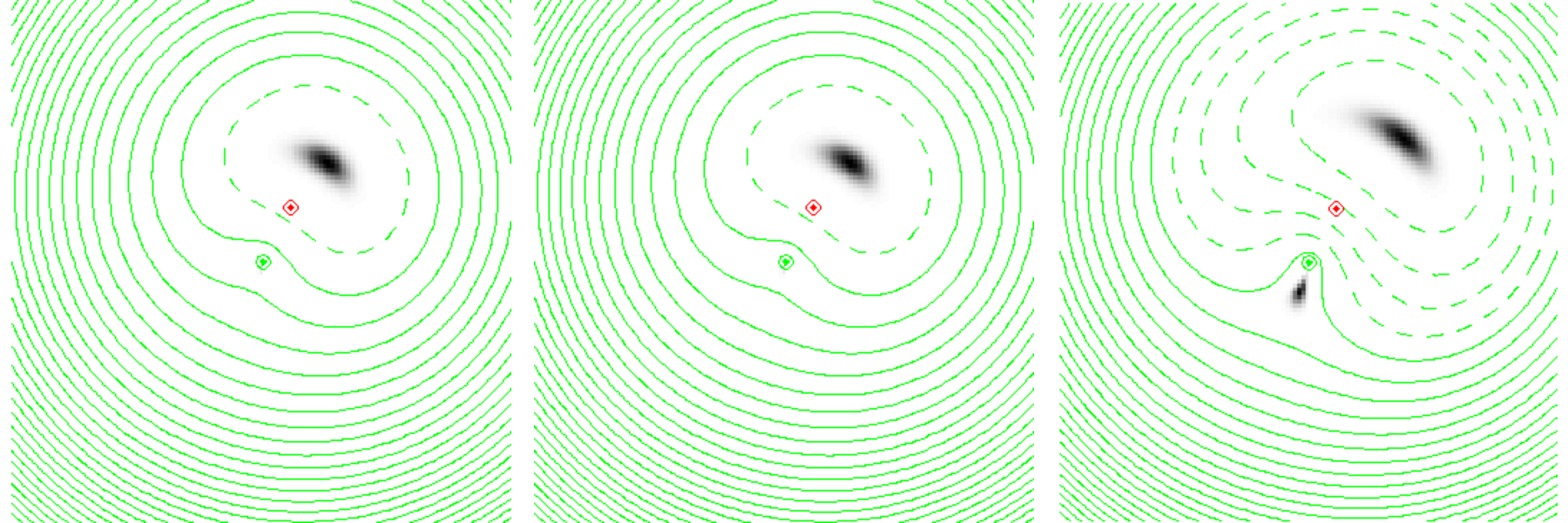
If we now allow the galaxy to have a steadily increasing mass, we introduce an extra time delay (known as the Shapiro delay) along light paths which pass through the lens plane close to the galaxy centre. This makes a distortion in the Fermat surface (Figure 3*). At first, its only effect is to displace the Fermat minimum away from the distortion. Eventually, however, the distortion becomes big enough to produce a maximum at the position of the galaxy, together with a saddle point on the other side of the galaxy from the minimum. By Fermat’s principle, two further images will appear at these two stationary points in the Fermat surface. This is the basic three-image lens configuration, although in practice the central image at the Fermat maximum is highly demagnified and not usually seen.
If the lens is significantly elliptical and the lines of sight are well aligned, we can produce five images, consisting of four images around a ring alternating between maxima and saddle points, and a central, highly demagnified Fermat maximum. Both four-image and two-image systems (“quads” and “doubles”) are in fact seen in practice. The major use of lens systems is for determining mass distributions in the lens galaxy, since the positions and fluxes of the images carry information about the gravitational potential of the lens. Gravitational lensing has the advantage that its effects are independent of whether the matter is light or dark, so in principle the effects of both baryonic and non-baryonic matter can be probed.
2.2.2 Principles of time delays
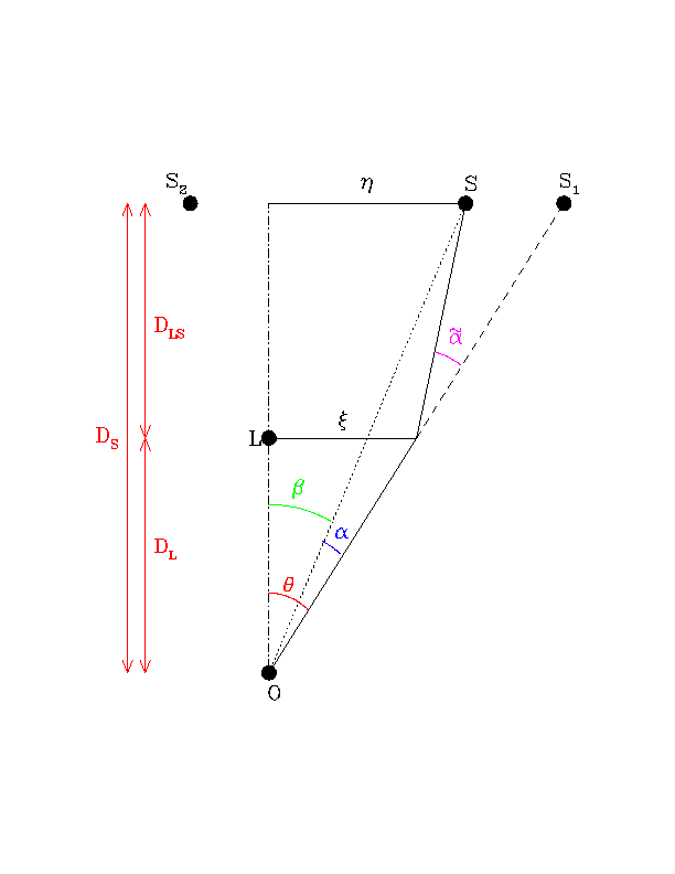
Refsdal [166] pointed out that if the background source is variable, it is possible to measure an absolute distance within the system and therefore the Hubble constant. To see how this works, consider the light paths from the source to the observer corresponding to the individual lensed images. Although each is at a stationary point in the Fermat time delay surface, the absolute light travel time for each will generally be different, with one of the Fermat minima having the smallest travel time. Therefore, if the source brightens, this brightening will reach the observer at different times corresponding to the two different light paths. Measurement of the time delay corresponds to measuring the difference in the light travel times, each of which is individually given by
where
 ,
,  and
and  are angles defined below in Figure 4*,
  ,
,  and
and  are angular diameter
distances also defined in Figure 4*,
are angular diameter
distances also defined in Figure 4*,  is the lens redshift, and
  is a term representing the Shapiro
delay of light passing through a gravitational field. Fermat’s principle corresponds to the requirement that
is a term representing the Shapiro
delay of light passing through a gravitational field. Fermat’s principle corresponds to the requirement that
 . Once the differential time delays are known, we can then calculate the ratio of angular diameter
distances which appears in the above equation. If the source and lens redshifts are known,
. Once the differential time delays are known, we can then calculate the ratio of angular diameter
distances which appears in the above equation. If the source and lens redshifts are known,  follows
from Eqs. 9* and 10*. The value derived depends on the geometric cosmological parameters
follows
from Eqs. 9* and 10*. The value derived depends on the geometric cosmological parameters  and
and  ,
but this dependence is relatively weak. A handy rule of thumb which can be derived from this
equation for the case of a 2-image lens, if we make the assumption that the matter distribution is
isothermal9
and
,
but this dependence is relatively weak. A handy rule of thumb which can be derived from this
equation for the case of a 2-image lens, if we make the assumption that the matter distribution is
isothermal9
and  , is
where
, is
where 
 is the lens redshift,
  is the separation of the images (approximately twice the Einstein radius),
 is the ratio of the fluxes and
  is the value of
  in Gpc. A larger time delay implies a
correspondingly lower
in Gpc. A larger time delay implies a
correspondingly lower  .
.
The first gravitational lens was discovered in 1979 [232] and monitoring programmes began soon
afterwards to determine the time delay. This turned out to be a long process involving a dispute between
proponents of a  400-day and a
  550-day delay, and ended with a determination of
417 ± 2 days [121*, 189]. Since that time, over 20 more time delays have been determined (see Table 1).
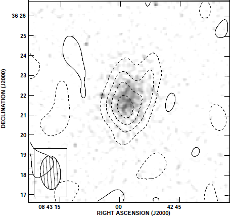
In the early days, many of the time delays were measured at radio wavelengths by examination of
those systems in which a radio-loud quasar was the multiply imaged source (see Figure 5*).
Recently, optically-measured delays have dominated, due to the fact that only a small optical
telescope in a site with good seeing is needed for the photometric monitoring, whereas radio time
delays require large amounts of time on long-baseline interferometers which do not exist in large
numbers.10
A time delay using
550-day delay, and ended with a determination of
417 ± 2 days [121*, 189]. Since that time, over 20 more time delays have been determined (see Table 1).
In the early days, many of the time delays were measured at radio wavelengths by examination of
those systems in which a radio-loud quasar was the multiply imaged source (see Figure 5*).
Recently, optically-measured delays have dominated, due to the fact that only a small optical
telescope in a site with good seeing is needed for the photometric monitoring, whereas radio time
delays require large amounts of time on long-baseline interferometers which do not exist in large
numbers.10
A time delay using  -rays has been determined for one lens [37*] using correlated variations in a
light-curve which contains emission from both images of the lens.
-rays has been determined for one lens [37*] using correlated variations in a
light-curve which contains emission from both images of the lens.
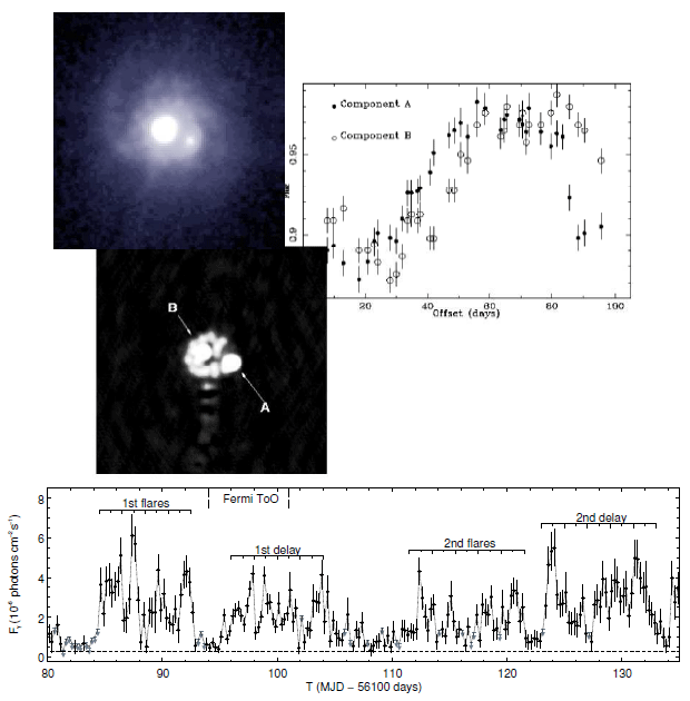
 -ray lightcurve [37*], in which, although the components are not resolved, the
sharpness of the variations allows a time delay to be determined (at 11.46 ± 0.16 days, significantly
greater than the radio time delay). Image reproduced with permission from [37]; copyright by AAS.
-ray lightcurve [37*], in which, although the components are not resolved, the
sharpness of the variations allows a time delay to be determined (at 11.46 ± 0.16 days, significantly
greater than the radio time delay). Image reproduced with permission from [37]; copyright by AAS.2.2.3 The problem with lens time delays
Unlike local distance determinations (and even unlike cosmological probes which
typically use more than one measurement), there is only one major systematic piece
of astrophysics in the determination of  by lenses, but it is a very important
one.11
This is the form of the potential in Eq. (11*). If one parametrises the potential in the form of a power law in
projected mass density versus radius, the index is
by lenses, but it is a very important
one.11
This is the form of the potential in Eq. (11*). If one parametrises the potential in the form of a power law in
projected mass density versus radius, the index is  for an isothermal model. This index has a pretty direct
degeneracy12
with the deduced length scale and therefore the Hubble constant; for a change of 0.1, the length scale
changes by about 10%. The sense of the effect is that a steeper index, which corresponds to a more centrally
concentrated mass distribution, decreases all the length scales and therefore implies a higher Hubble
constant for a given time delay.
for an isothermal model. This index has a pretty direct
degeneracy12
with the deduced length scale and therefore the Hubble constant; for a change of 0.1, the length scale
changes by about 10%. The sense of the effect is that a steeper index, which corresponds to a more centrally
concentrated mass distribution, decreases all the length scales and therefore implies a higher Hubble
constant for a given time delay.
If an uncertainty in the slope of a power-law mass distribution were the only issue, then this could be
constrained by lensing observables in the case where the source is extended, resulting in measurements of
lensed structure at many different points in the lens plane [115]. This has been done, for example, using
multiple radio sources [38], VLBI radio structure [239] and in many objects using lensed structure of
background galaxies [21], although in this latter case  is not measurable because the background
objects are not variable. The degeneracy between the Hubble constant and the mass model is
more general than this, however [76]. The reason is that lensing observables give information
about the derivatives of the Fermat surface; the positions of the images are determined by
the first derivatives of the surface, and the fluxes by the second derivatives. For any given set
of lensing observables, we can move the intrinsic source position, thus changing the Fermat
surface, and then restore the observables to their original values by adjusting the mass model and
thus returning the Fermat surface to its original configuration. It therefore follows that any
given set of measurements of image positions and fluxes in a lens system is consistent with a
number of different mass models, and therefore a number of different values of
is not measurable because the background
objects are not variable. The degeneracy between the Hubble constant and the mass model is
more general than this, however [76]. The reason is that lensing observables give information
about the derivatives of the Fermat surface; the positions of the images are determined by
the first derivatives of the surface, and the fluxes by the second derivatives. For any given set
of lensing observables, we can move the intrinsic source position, thus changing the Fermat
surface, and then restore the observables to their original values by adjusting the mass model and
thus returning the Fermat surface to its original configuration. It therefore follows that any
given set of measurements of image positions and fluxes in a lens system is consistent with a
number of different mass models, and therefore a number of different values of  , because
the source position cannot be determined. Therefore the assumption of a particular type of
model, such as a power-law, itself constitutes a selection of a particular one out of a range of
possible models [192], each of which would give a different
, because
the source position cannot be determined. Therefore the assumption of a particular type of
model, such as a power-law, itself constitutes a selection of a particular one out of a range of
possible models [192], each of which would give a different  . Modelling degeneracies arise
not only from the mass distribution within the lens galaxy, but also from matter along the
line of sight. These operate in the sense that, if a mass sheet is present which is not known
about, the length scale obtained is too short and consequently the derived value of
. Modelling degeneracies arise
not only from the mass distribution within the lens galaxy, but also from matter along the
line of sight. These operate in the sense that, if a mass sheet is present which is not known
about, the length scale obtained is too short and consequently the derived value of  is too
high.
is too
high.
There are a number of approaches to this mass-degeneracy problem. The first is to use a non-parametric model for the projected mass distribution, imposing only a minimum number of physically-motivated requirements such as monotonicity, and thereby generate large numbers of mass models which are exactly consistent with the data. This was pioneered by Saha and Williams in a series of papers [179, 237, 180, 177*] in which pixellated models of galaxy mass distributions were used. Although pixellated models are useful for exploring the space of allowed models, they do not break the essential degeneracy. Other priors may be used, however: in principle it should also be possible to reject some possible mass distributions on physical grounds, because we expect the mass profiles to contain a central stellar cusp and a more extended dark matter halo. Undisturbed dark matter haloes should have profiles similar to a Navarro, Frenk & White (NFW, [139]) form, but they may be modified by adiabatic contraction during the process of baryonic infall when the galaxy forms.
Second, it is possible to increase the reliability of individual lens mass models by gathering extra
information which partially breaks the mass degeneracy. A major improvement is available by the use of
stellar velocity dispersions [221*, 220, 222, 119*] measured in the lensing galaxy. As a standalone
determinant of mass models in galaxies at  , typical of lens galaxies, such measurements are not
very useful as they suffer from severe degeneracies with the structure of stellar orbits. However, the
combination of lensing information (which gives a very accurate measurement of mass enclosed by the
Einstein radius) and stellar dynamics (which gives, more or less, the mass enclosed within the effective
radius of the stellar light) gives a measurement that in effect selects only some of the family of
possible lens models which fit a given set of lensing observables. The method has large error
bars, in part due to residual dependencies on the shape of stellar orbits, but also because these
measurements are very difficult; each galaxy requires about one night of good seeing on a 10-m
telescope. Nevertheless, this programme has the potential beneficial effect of reducing the dominant
systematic error, despite the potential additional systematic from the assumptions about stellar
orbits.
, typical of lens galaxies, such measurements are not
very useful as they suffer from severe degeneracies with the structure of stellar orbits. However, the
combination of lensing information (which gives a very accurate measurement of mass enclosed by the
Einstein radius) and stellar dynamics (which gives, more or less, the mass enclosed within the effective
radius of the stellar light) gives a measurement that in effect selects only some of the family of
possible lens models which fit a given set of lensing observables. The method has large error
bars, in part due to residual dependencies on the shape of stellar orbits, but also because these
measurements are very difficult; each galaxy requires about one night of good seeing on a 10-m
telescope. Nevertheless, this programme has the potential beneficial effect of reducing the dominant
systematic error, despite the potential additional systematic from the assumptions about stellar
orbits.
Third, we can remove problems associated with mass sheets associated with material extrinsic to the main lensing galaxy by measuring them using detailed studies of the environments of lens galaxies. Studies of lens groups [60, 106, 59, 137] show that neglecting matter along the line of sight typically has an effect of 10 – 20%, with matter close to the redshift of the lens contributing most. More recently, it has been shown that a combination of studies of number counts and redshifts of nearby objects to the main lens galaxy, coupled with comparisons to large numerical simulations of matter such as the Millenium Simulation, can reduce the errors associated with the environment to around 3 – 4% [78].
2.2.4 Time delay measurements
Table 1 shows the currently measured time delays, with references and comments. The addition of new measurements is now occurring at a much faster rate, due to the advent of more systematic dedicated monitoring programmes, in particular that of the COSMOGRAIL collaboration (e.g., [230*, 231*, 41*, 164*, 57*]). Considerable patience is needed for these efforts in order to determine an unambiguous delay for any given object, given the contaminating effects of microlensing and also the unavoidable gaps in the monitoring schedule (at least for optical monitoring programmes) once per year as the objects move into the daytime. Derivation of time delays under these circumstances is not a trivial matter, and algorithms which can cope with these effects have been under continuous development for decades [156, 114, 88, 217*] culminating in a blind analysis challenge [50].
 errors, from the literature. In some cases multiple delays have
been measured in 4-image lens systems, and in this case each delay is given separately for the two
components in brackets. An additional time delay for CLASS B1422+231 [151] probably requires
verification, and a published time delay for Q0142–100 [120, 146] has large errors. Time delays for
the CLASS and PKS objects have been obtained using radio interferometers, and the remainder
using optical telescopes.
errors, from the literature. In some cases multiple delays have
been measured in 4-image lens systems, and in this case each delay is given separately for the two
components in brackets. An additional time delay for CLASS B1422+231 [151] probably requires
verification, and a published time delay for Q0142–100 [120, 146] has large errors. Time delays for
the CLASS and PKS objects have been obtained using radio interferometers, and the remainder
using optical telescopes.| Lens system |
Time delay
|
Reference |
|
[days]
|
||
| CLASS 0218+357 |  |
[16] |
| HE 0435-1-223 |  (AD) (AD) |
[116] |
 (BC) (BC) |
also others [41] | |
| SBS 0909+532 |  ( ( ) ) |
[229] |
| RX 0911+0551 |  |
[86] |
| FBQ 0951+2635 |  |
[103] |
| Q 0957+561 |  |
[121] |
| SDSS 1001+5027 |  |
[164] |
| SDSS 1004+4112 |  (AB) (AB) |
[65] |
| SDSS 1029+2623 | [64] | |
| HE 1104–185 |  |
[140] |
| PG 1115+080 |  (BC) (BC) |
[188] |
 (AC) (AC) |
||
| RX 1131–1231 |  (AB) (AB) |
[138] |
 (AC) (AC) |
||
 (AD) (AD) |
||
| [217] | ||
| SDSS J1206+4332 |  |
[57*] |
| SBS 1520+530 |  |
[30] |
| CLASS 1600+434 |  |
[28] |
 |
[118] | |
| CLASS 1608+656 |  (AB) (AB) |
[61] |
 (BC) (BC) |
||
 (BD) (BD) |
||
| SDSS 1650+4251 |  |
[230] |
| PKS 1830–211 |  |
[127] |
| WFI J2033–4723 |  (AB) (AB) |
[231] |
| HE 2149–2745 |  |
[29] |
| HS 2209+1914 |  |
[57] |
| Q 2237+0305 |  |
[44] |
2.2.5 Derivation of H0: Now, and the future
Initially, time delays were usually turned into Hubble constant values using assumptions about the mass
model – usually that of a single, isothermal power law [119] – and with rudimentary modelling of the
environment of the lens system as necessary. Early analyses of this type resulted in rather low values of the
Hubble constant [112] for some systems, sometimes due to the steepness of the lens potential [221]. As the
number of measured time delays expanded, combined analyses of multiple lens systems were conducted,
often assuming parametric lens models [141*] but also using Monte Carlo methods to account for quantities
such as the presence of clusters around the main lens. These methods typically give values around
 – e.g., (
 from Oguri (2007) [141], but with an
uncomfortably greater spread between lens systems than would be expected on the basis of the formal
errors. An alternative approach to composite modelling is to use non-parametric lens models, on the
grounds that these may permit a wider range of mass distributions [177*, 150*] even though they also
contain some level of prior assumptions. Saha et al. (2006) [177] used ten time-delay lenses for this
purpose, and Paraficz et al. (2010) [150] extended the analysis to eighteen systems obtaining
from Oguri (2007) [141], but with an
uncomfortably greater spread between lens systems than would be expected on the basis of the formal
errors. An alternative approach to composite modelling is to use non-parametric lens models, on the
grounds that these may permit a wider range of mass distributions [177*, 150*] even though they also
contain some level of prior assumptions. Saha et al. (2006) [177] used ten time-delay lenses for this
purpose, and Paraficz et al. (2010) [150] extended the analysis to eighteen systems obtaining
 , with a further extension by Sereno & Paraficz (2014) [194*] giving
  (stat/syst) km s−1 Mpc−1.
In the last few years, concerted attempts have emerged to put together improved time-delay observations
with systematic modelling. For two existing time-delay lenses (CLASS B1608+656 and
RXJ 1131–1231) modelling has been undertaken [205, 206*] using a combination of all of the previously
described ingredients: stellar velocity dispersions to constrain the lens model and partly break the mass
degeneracy, multi-band HST imaging to evaluate and model the extended light distribution of the lensed
object, comparison with numerical simulations to gauge the likely contribution of the line of sight to the
lensing potential, and the performance of the analysis blind (without sight of the consequences for  of
any decision taken during the modelling). The results of the two lenses together,
of
any decision taken during the modelling). The results of the two lenses together,  and
and  in flat and open
  CDM, respectively, are probably the most
reliable determinations of
CDM, respectively, are probably the most
reliable determinations of  from lensing to date, even if they do not have the lowest formal
error13.
from lensing to date, even if they do not have the lowest formal
error13.
In the immediate future, the most likely advances come from further analysis of existing time delay
lenses, although the process of obtaining the data for good quality time delays and constraints on the mass
model is not a quick process. A number of further developments will expedite the process. The first is the
likely discovery of lenses on an industrial scale using the Large Synoptic Survey Telescope (LSST, [101]) and
the Euclid satellite [4], together with time delays produced by high cadence monitoring. The second is the
availability in a few years’ time of  8-m class optical telescopes, which will ease the followup
problem considerably. A third possibility which has been discussed in the past is the use of
double source-plane lenses, in which two background objects, one of which is a quasar, are
imaged by a single foreground object [74, 39]. Unfortunately, it appears [191] that even this
additional set of constraints leave the mass degeneracy intact, although it remains to be seen
whether dynamical information will help relatively more in these objects than in single-plane
systems.
8-m class optical telescopes, which will ease the followup
problem considerably. A third possibility which has been discussed in the past is the use of
double source-plane lenses, in which two background objects, one of which is a quasar, are
imaged by a single foreground object [74, 39]. Unfortunately, it appears [191] that even this
additional set of constraints leave the mass degeneracy intact, although it remains to be seen
whether dynamical information will help relatively more in these objects than in single-plane
systems.
One potentially clean way to break mass model degeneracies is to discover a lensed type Ia supernova [142, 143*]. The reason is that, as we have seen, the intrinsic brightness of SNe Ia can be determined from their lightcurve, and it can be shown that the resulting absolute magnification of the images can then be used to bypass the effective degeneracy between the Hubble constant and the radial mass slope. Oguri et al. [143] and also Bolton and Burles [20] discuss prospects for finding such objects; future surveys with the Large Synoptic Survey Telescope (LSST) are likely to uncover significant numbers of such events. The problem is likely to be the determination of the time delay, since nearly all such objects are subject to significant microlensing effects within the lensing galaxy which is likely to restrict the accuracy of the measurement [51].
2.3 The Sunyaev–Zel’dovich effect
The basic principle of the Sunyaev–Zel’dovich (S-Z) method [203], including its use to determine the
Hubble constant [196], is reviewed in detail in [18*, 33]. It is based on the physics of hot ( ) gas in
clusters, which emits X-rays by bremsstrahlung emission with a surface brightness given by the equation
(see e.g., [18])
) gas in
clusters, which emits X-rays by bremsstrahlung emission with a surface brightness given by the equation
(see e.g., [18])

 is the electron density and
  the spectral emissivity, which depends on the electron
temperature.
the spectral emissivity, which depends on the electron
temperature.
At the same time, the electrons of the hot gas in the cluster Compton upscatter photons from the CMB radiation. At radio frequencies below the peak of the Planck distribution, this causes a “hole” in radio emission as photons are removed from this spectral region and turned into higher-frequency photons (see Figure 6*). The decrement is given by an optical-depth equation,
involving many of the same parameters and a function
 which depends on frequency and
electron temperature. It follows that, if both
which depends on frequency and
electron temperature. It follows that, if both  and
and  can be measured, we have two
equations for the variables
can be measured, we have two
equations for the variables  and the integrated length
  through the cluster and can
calculate both quantities. Finally, if we assume that the projected size
through the cluster and can
calculate both quantities. Finally, if we assume that the projected size  of the cluster on the
sky is equal to
of the cluster on the
sky is equal to  , we can then derive an angular diameter distance if we know the angular
size of the cluster. The Hubble constant is then easy to calculate, given the redshift of the
cluster.
, we can then derive an angular diameter distance if we know the angular
size of the cluster. The Hubble constant is then easy to calculate, given the redshift of the
cluster.
 using the S-Z effect. Model types are
  for the
assumption of a
for the
assumption of a  -model and H for a hydrostatic equilibrium model. Some of the studies target
the same clusters, with three objects being common to more than one of the four smaller studies,
The larger study [22*] contains four of the objects from [104*] and two from [190*].
-model and H for a hydrostatic equilibrium model. Some of the studies target
the same clusters, with three objects being common to more than one of the four smaller studies,
The larger study [22*] contains four of the objects from [104*] and two from [190*]. determination
 ]
]


Although in principle a clean, single-step method, in practice there are a number of possible
difficulties. Firstly, the method involves two measurements, each with a list of possible errors. The
X-ray determination carries a calibration uncertainty and an uncertainty due to absorption
by neutral hydrogen along the line of sight. The radio observation, as well as the calibration,
is subject to possible errors due to subtraction of radio sources within the cluster which are
unrelated to the S-Z effect. Next, and probably most importantly, are the errors associated with
the cluster modelling. In order to extract parameters such as electron temperature, we need
to model the physics of the X-ray cluster. This is not as difficult as it sounds, because X-ray
spectral information is usually available, and line ratio measurements give diagnostics of physical
parameters. For this modelling the cluster is usually assumed to be in hydrostatic equilibrium, or a
“beta-model” (a dependence of electron density with radius of the form  ) is
assumed. Several recent works [190, 22*] relax this assumption, instead constraining the profile
of the cluster with available X-ray information, and the dependence of
) is
assumed. Several recent works [190, 22*] relax this assumption, instead constraining the profile
of the cluster with available X-ray information, and the dependence of  on these details
is often reassuringly small (
on these details
is often reassuringly small ( ). Finally, the cluster selection can be done carefully to
avoid looking at prolate clusters along the long axis (for which
). Finally, the cluster selection can be done carefully to
avoid looking at prolate clusters along the long axis (for which  ) and therefore seeing
more X-rays than one would predict. This can be done by avoiding clusters close to the flux
limit of X-ray flux-limited samples, Reese et al. [165] estimate an overall random error budget
of 20 – 30% for individual clusters. As in the case of gravitational lenses, the problem then
becomes the relatively trivial one of making more measurements, provided there are no unforeseen
systematics.
) and therefore seeing
more X-rays than one would predict. This can be done by avoiding clusters close to the flux
limit of X-ray flux-limited samples, Reese et al. [165] estimate an overall random error budget
of 20 – 30% for individual clusters. As in the case of gravitational lenses, the problem then
becomes the relatively trivial one of making more measurements, provided there are no unforeseen
systematics.
The cluster samples of the most recent S-Z determinations (see Table 2) are not independent in that
different authors often observe the same clusters. The most recent work, that in [22*] is larger than
the others and gives a higher  . It is worth noting, however, that if we draw subsamples
from this work and compare the results with the other S-Z work, the
. It is worth noting, however, that if we draw subsamples
from this work and compare the results with the other S-Z work, the  values from the
subsamples are consistent. For example, the
values from the
subsamples are consistent. For example, the  derived from the data in [22] and modelling of the
five clusters also considered in [104*] is actually lower than the value of
derived from the data in [22] and modelling of the
five clusters also considered in [104*] is actually lower than the value of  in [104]. Within the smaller samples, the scatter is much lower than the quoted errors, partially
due to the overlap in samples (three objects are common to more than one of the four smaller
studies).
in [104]. Within the smaller samples, the scatter is much lower than the quoted errors, partially
due to the overlap in samples (three objects are common to more than one of the four smaller
studies).
It therefore seems as though S-Z determinations of the Hubble constant are beginning to converge to a
value of around  , although the errors are still large, values in the low to mid-sixties are
still consistent with the data and it is possible that some objects may have been observed but not used to
derive a published
, although the errors are still large, values in the low to mid-sixties are
still consistent with the data and it is possible that some objects may have been observed but not used to
derive a published  value. Even more than in the case of gravitational lenses, measurements of
 from individual clusters are occasionally discrepant by factors of nearly two in either
direction, and it would probably teach us interesting astrophysics to investigate these cases
further.
from individual clusters are occasionally discrepant by factors of nearly two in either
direction, and it would probably teach us interesting astrophysics to investigate these cases
further.
2.4 Gamma-ray propagation
High-energy  -rays emitted by distant AGN are subject to interactions with ambient photons
during their passage towards us, producing electron-positron pairs. The mean free path for
this process varies with photon energy, being smaller at higher energies, and is generally a
substantial fraction of the distance to the sources. The observed spectrum of
-rays emitted by distant AGN are subject to interactions with ambient photons
during their passage towards us, producing electron-positron pairs. The mean free path for
this process varies with photon energy, being smaller at higher energies, and is generally a
substantial fraction of the distance to the sources. The observed spectrum of  -ray sources
therefore shows a high-energy cutoff, whose characteristic energy decreases with increasing
redshift. The expected cutoff, and its dependence on redshift, has been detected with the Fermi
satellite [1].
-ray sources
therefore shows a high-energy cutoff, whose characteristic energy decreases with increasing
redshift. The expected cutoff, and its dependence on redshift, has been detected with the Fermi
satellite [1].
The details of this effect depend on the Hubble constant, and can therefore be used to measure
it [183, 11]. Because it is an optical depth effect, knowledge of the interaction cross-section from basic
physics, together with the number density  of the interacting photons, allows a length measurement
and, assuming knowledge of the redshift of the source,
of the interacting photons, allows a length measurement
and, assuming knowledge of the redshift of the source,  . In practice, the cosmological world model
is also needed to determine
. In practice, the cosmological world model
is also needed to determine  from observables. From the existing Fermi data a value of
 is estimated [52] although the errors, dominated by the calculation of the evolution of
the extragalactic background light using galaxy luminosity functions and spectral energy distributions, are
currently quite large (
is estimated [52] although the errors, dominated by the calculation of the evolution of
the extragalactic background light using galaxy luminosity functions and spectral energy distributions, are
currently quite large ( ).
).
 |
 |
 |