List of Figures
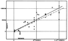 |
Figure 1:
Hubble’s original diagram of distance to nearby galaxies, derived from measurements using Cepheid variables, against velocity, derived from redshift. The Hubble constant is the slope of this relation, and in this diagram is a factor of nearly 10 steeper than currently accepted values. Image reproduced from [95]. |
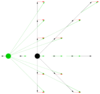 |
Figure 2:
Illustration of the Hubble law. Galaxies at all points of the square grid are receding from the black galaxy at the centre, with velocities proportional to their distance away from it. From the point of view of the second, green, galaxy two grid points to the left, all velocities are modified by vector addition of its velocity relative to the black galaxy (red arrows). When this is done, velocities of galaxies as seen by the second galaxy are indicated by green arrows; they all appear to recede from this galaxy, again with a Hubble-law linear dependence of velocity on distance. |
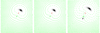 |
Figure 3:
Illustration of a Fermat surface for a source (red symbol) close to the line of sight to a galaxy (green symbol). In each case the appearance of the images to the observer is shown by a greyscale, and the contours of the Fermat surface are given by green contours. Note that images form at stationary points of the surface defined by the contours. In the three panels, the mass of the galaxy, and thus the distortion of the Fermat surface, increases, resulting in an increasingly visible secondary image at the position of the saddle point. At the same time, the primary image moves further from the line of sight to the source. In each case the third image, at the position of the Fermat maximum, is too faint to see. |
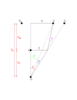 |
Figure 4:
Basic geometry of a gravitational lens system. Image reproduced from [233]; copyright by the author. |
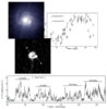 |
Figure 5:
The lens system JVAS B0218+357. Top right: the measurement of time delay of about 10 days from asynchronous variations of the two lensed images [16]. The upper left panels show the HST/ACS image [241] on which can be seen the two images and the spiral lensing galaxy, and the radio MERLIN+VLA image [17] showing the two images together with an Einstein ring. The bottom panel shows the  -ray lightcurve [37], in which, although the components are not resolved, the
sharpness of the variations allows a time delay to be determined (at 11.46 ± 0.16 days, significantly
greater than the radio time delay). Image reproduced with permission from [37]; copyright by AAS. -ray lightcurve [37], in which, although the components are not resolved, the
sharpness of the variations allows a time delay to be determined (at 11.46 ± 0.16 days, significantly
greater than the radio time delay). Image reproduced with permission from [37]; copyright by AAS. |
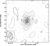 |
Figure 6:
S-Z decrement observation of Abell 697 with the Ryle telescope in contours superimposed on the ROSAT image (grey-scale). Image reproduced with permission from [104]; copyright by RAS. |
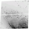 |
Figure 7:
Positions of Cepheid variables in HST/ACS observations of the galaxy NGC 4258. Typical Cepheid lightcurves are shown on the top. Image reproduced with permission from [129]; copyright by AAS. |
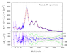 |
Figure 8:
Diagram of the CMB anisotropies, plotted as strength against spatial frequency, from the 2013 Planck data. The measured points are shown together with best-fit models. Note the acoustic peaks, the largest of which corresponds to an angular scale of about half a degree. Image reproduced with permission from [2], copyright by ESO. |
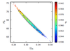 |
Figure 9:
The allowed range of the parameters  , ,  , from the 2013 Planck data, is shown as
a series of points. A flat Universe is assumed, together with information from the Planck fluctuation
temperature spectrum, CMB lensing information from Planck, and WMAP polarization observations.
The colour coding reflects different values of , from the 2013 Planck data, is shown as
a series of points. A flat Universe is assumed, together with information from the Planck fluctuation
temperature spectrum, CMB lensing information from Planck, and WMAP polarization observations.
The colour coding reflects different values of  , the spectral index of scalar perturbations as a
function of spatial scale at early times. Image reproduced with permission from [2], copyright by
ESO. , the spectral index of scalar perturbations as a
function of spatial scale at early times. Image reproduced with permission from [2], copyright by
ESO. |