4 The CMB and Cosmological Estimates of the Distance Scale

4.1 The physics of the anisotropy spectrum and its implications

The physics of stellar distance calibrators is very complicated, because it comes from the era in which the Universe has had time to evolve complicated astrophysics. A large class of alternative approaches to cosmological parameters in general involve going back to an era where astrophysics is relatively simple and linear, the epoch of recombination at which the CMB fluctuations can be studied. Although tests involving the CMB do not directly determine , they provide joint information about and other cosmological parameters which is improving at a very rapid rate.

In the Universe’s early history, its temperature was high enough to prohibit the formation of atoms, and the Universe was therefore ionized. Approximately after the Big Bang, corresponding to a redshift , the temperature dropped enough to allow the formation of atoms, a point known as “recombination”. For photons, the consequence of recombination was that photons no longer scattered from ionized particles but were free to stream. After recombination, these primordial photons reddened with the expansion of the Universe, forming the cosmic microwave background (CMB) which we observe today as a black-body radiation background at 2.73 K.

In the early Universe, structure existed in the form of small density fluctuations () in the photon-baryon fluid. The resulting pressure gradients, together with gravitational restoring forces, drove oscillations, very similar to the acoustic oscillations commonly known as sound waves. Fluctuations prior to recombination could propagate at the relativistic () sound speed as the Universe expanded. At recombination, the structure was dominated by those oscillation frequencies which had completed a half-integral number of oscillations within the characteristic size of the Universe at recombination;¹⁹ this pattern became frozen into the photon field which formed the CMB once the photons and baryons decoupled and the sound speed dropped. The process is reviewed in much more detail in [92].

The resulting “acoustic peaks” dominate the fluctuation spectrum (see Figure 8*). Their angular scale is a function of the size of the Universe at the time of recombination, and the angular diameter distance between us and . Since the angular diameter distance is a function of cosmological parameters, measurement of the positions of the acoustic peaks provides a constraint on cosmological parameters. Specifically, the more closed the spatial geometry of the Universe, the smaller the angular diameter distance for a given redshift, and the larger the characteristic scale of the acoustic peaks. The measurement of the peak position has become a strong constraint in successive observations (in particular BOOMERanG [47], MAXIMA [83], and WMAP, reported in [201*] and [202*]) and corresponds to an approximately spatially flat Universe in which .

Figure 8: Diagram of the CMB anisotropies, plotted as strength against spatial frequency, from the 2013 Planck data. The measured points are shown together with best-fit models. Note the acoustic peaks, the largest of which corresponds to an angular scale of about half a degree. Image reproduced with permission from [2*], copyright by ESO.

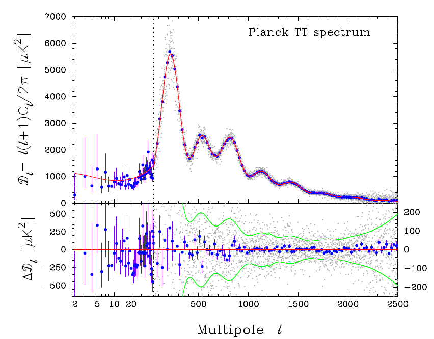
But the global geometry of the Universe is not the only property which can be deduced from the fluctuation spectrum.²⁰ The peaks are also sensitive to the density of baryons, of total (baryonic + dark) matter, and of vacuum energy (energy associated with the cosmological constant). These densities scale with the square of the Hubble parameter times the corresponding dimensionless densities [see Eq. (5*)] and measurement of the acoustic peaks therefore provides information on the Hubble constant, degenerate with other parameters, principally and . The second peak strongly constrains the baryon density, , and the third peak is sensitive to the total matter density in the form .

4.2 Degeneracies and implications for H₀

Although the CMB observations provide significant information about cosmological parameters, the available data constrain combinations of with other parameters, and either assumptions or other data must be provided in order to derive the Hubble constant. One possible assumption is that the Universe is exactly flat (i.e., ) and the primordial fluctuations have a power law spectrum. In this case measurements of the CMB fluctuation spectrum with the Wilkinson Anisotropy Probe (WMAP) satellite [201, 202*] and more recently with the Planck satellite [2*], allow to be derived. This is because measuring produces a locus in the plane which is different from the locus of the flat Universe, and although the tilt of these two lines is not very different, an accurate CMB measurement can localise the intersection enough to give and separately. The value of was derived in this way by WMAP [202] and, using the more accurate spectrum provided by Planck, as  [2*]. In this case, other cosmological parameters can be determined to two and in some cases three significant figures,²¹ Figure 9* shows this in another way, in terms of as a function of in a flat universe [ in Eq. (10*)].

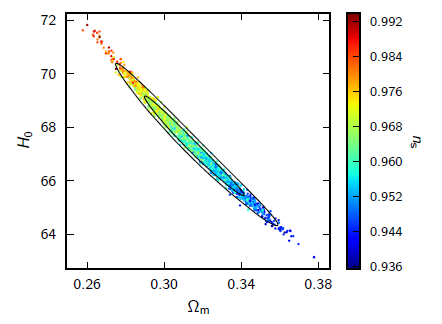
Figure 9: The allowed range of the parameters , , from the 2013 Planck data, is shown as a series of points. A flat Universe is assumed, together with information from the Planck fluctuation temperature spectrum, CMB lensing information from Planck, and WMAP polarization observations. The colour coding reflects different values of , the spectral index of scalar perturbations as a function of spatial scale at early times. Image reproduced with permission from [2*], copyright by ESO.

If we do not assume the universe to be exactly flat, as is done in Figure 9*, then we obtain a degeneracy with in the sense that decreasing increases the total density of the universe (approximately by 0.1 in units of the critical density for a 20 km s−1 Mpc−1 decrease in ). CMB data by themselves, without any further assumptions or extra data, do not supply a significant constraint on compared to those which are obtainable by other methods. Other observing programmes are, however, available which result in constraints on the Hubble constant together with other parameters, notably , and (the dark energy equation of state parameter defined in Section 1.2); we can either regard as a constant or allow a variation with redshift. We sketch these briefly here; a full review of all programmes addressing cosmic acceleration can be found in the review by Weinberg et al. [235*].

The first such supplementary programme is the study of type Ia supernovae, which as we have seen function as standard candles (or at least easily calibratable candles). They therefore determine the luminosity distance . Studies of SNe Ia were the first indication that varies with in such a way that an acceleration term, corresponding to a non-zero is required [157, 158, 169], a discovery that won the 2011 Nobel Prize in physics. This determination of luminosity distance gives constraints in the plane, which are more or less orthogonal to the CMB constraints. Currently, the most complete samples of distant SNe come from SDSS surveys at low redshift () [73, 182, 89, 109], the ESSENCE survey at moderate redshift () [135, 238], the SNLS surveys at  [40] and high-redshift () HST surveys [171, 46, 208]. In the future, surveys in the infrared should be capable of extending the redshift range further [175].

The second important programme is the measurement of structure at more recent epochs than the epoch of recombination using the characteristic length scale frozen into the structure of matter at recombination (Section 4.1). This is manifested in the real Universe by an expected preferred correlation length of  100 Mpc between observed baryon structures, otherwise known as galaxies. These baryon acoustic oscillations (BAOs) measure a standard rod, and constrain the distance measure (e.g. [56*]). The largest sample available for such studies comes from luminous red galaxies (LRGs) in the Sloan Digital Sky Survey [240]. The expected signal was first found [56] in the form of an increased power in the cross-correlation between galaxies at separations of about 100 Mpc, and corresponds to an effective measurement of angular diameter distance to a redshift . Since then, this characteristic distance has been found in other samples at different redshifts, 6dFGS at  [15*], further SDSS work at  [148*] and by the BOSS and WiggleZ collaborations at  [19*, 6*]. It has also been observed in studies of the Ly forest [31, 199, 48]. In principle, provided the data are good enough, the BAO can be studied separately in the radial and transverse directions, giving separate constraints on and  [184, 26] and hence more straightforward and accurate cosmology.

There are a number of other programmes that constrain combinations of cosmological parameters, which can break degeneracies involving . Weak-lensing observations have progressed very substantially over the last decade, after a large programme of quantifying and reducing systematic errors; these observations consist of measuring shapes of large numbers of galaxies in order to extract the small shearing signal produced by matter along the line of sight. The quantity directly probed by such observations is a combination of and , the rms density fluctuation at a scale of . State-of-the-art surveys include the CFHT survey [85, 110] and SDSS-based surveys [125]. Structure can also be mapped using Lyman- forest observations. The spectra of distant quasars have deep absorption lines corresponding to absorbing matter along the line of sight. The distribution of these lines measures clustering of matter on small scales and thus carries cosmological information (e.g. [226, 133]). Clustering on small scales [215] can be mapped, and the matter power spectrum can be measured, using large samples of galaxies, giving constraints on combinations of , and .

4.2.1 Combined constraints

As already mentioned, Planck observations of the CMB alone are capable of supplying a good constraint on , given three assumptions: the curvature of the Universe, , is zero, that dark energy is a cosmological constant () and that it is independent of redshift (). In general, every other accurate measurement of a combination of cosmological parameters allows one to relax one of the assumptions. For example, if we admit the BAO data together with the CMB, we can allow to be a free parameter [216, 6*, 2*]. Using earlier WMAP data for the CMB, is derived to be  [134, 6*], which does not change significantly using Planck data ( [2*]); the curvature in each case is tightly constrained (to ) and consistent with zero. If we introduce supernova data instead of BAO data, we can obtain provided that  [235*, 2*] and this is found to be consistent with within errors of about 0.1 – 0.2 [2*].

If we wish to proceed further, we need to introduce additional data to get tight constraints on . The obvious option is to use both BAO and SNe data together with the CMB, which results in  [19*] and (see Table 4 of [6*]) using the WMAP CMB constraints. Such analyses continue to give low errors on even allowing for a varying in a non-flat universe, although they do use the results from three separate probes to achieve this. Alternatively, extrapolation of the BAO results to give directly [55, 15*, 235] because the BAO measures a standard ruler, and the lower the redshift, the purer the standard ruler’s dependence on the Hubble constant becomes, independent of other elements in the definition of Hubble parameter such as and . The lowest-redshift BAO measurement is that of the 6dF, which suggests  [15*].