3 Searches for Gravitational-Wave Transients

Data from GW detectors are searched for many types of possible signals [8]. Here we focus on signals from compact binary coalescences (CBCs), including BNS systems, and on generic transient or burst signals. See [19*, 18*, 14*] for observational results from LIGO and Virgo for such systems.

The rate of BNS coalescences is uncertain [54]. For this work we adopt the estimates of [13*], which predicts the rate to lie between – , with a most plausible value of ; this corresponds to 0.4 – 400 signals above an SNR of 8 per year of observation for a single aLIGO detector at final sensitivity, and a best estimate of 40 BNS signals per year [13*]. Rate estimation remains an active area of research (e.g., [69, 50, 49, 47]), and will be informed by the number of detections (or lack thereof) in observing runs.

While the intrinsic rates of neutron star–black hole (NS–BH) and binary black hole (BBH) mergers are expected to be a factor of tens or hundreds lower than the BNS rate, the distance to which they can be observed is a factor of two to five larger. Consequently, the predicted observable rates are similar [13*, 92]. Expected rates for other transient sources are lower and/or less well constrained.

The gravitational waveform from a BNS coalescence is well modeled and matched filtering can be used to search for signals and measure the system parameters [74, 35, 34*, 90]. For systems containing black holes, or in which the component spin is significant, uncertainties in the waveform model can reduce the sensitivity of the search [81, 62, 45, 103, 85, 95, 68]. Searches for bursts make few assumptions on the signal morphology, using time–frequency decompositions to identify statistically significant excess-power transients in the data. Burst searches generally perform best for short-duration signals ( 1 s), although search development remains an area of active research (e.g., [71*, 102, 40, 106, 26, 104, 43*, 105, 66*]); their astrophysical targets include core-collapse supernovae, magnetar flares, BBH coalescences, cosmic string cusps, and, possibly, as-yet-unknown systems.

In the era of advanced detectors, the LSC and Virgo will search in near real-time for CBC and burst signals for the purpose of rapidly identifying event candidates. A prompt notice of a potential GW transient by LIGO–Virgo might enable follow-up observations in the electromagnetic spectrum. A first follow-up program including low-latency analysis, event candidate selection, position reconstruction and the sending of alerts to several observing partners (optical, X-ray, and radio) was implemented and exercised during the 2009 – 2010 LIGO–Virgo science run [16*, 15*, 53]. Latencies of less than 1 hour were achieved and we expect to improve this in the advanced-detector era. Increased detection confidence, improved sky localization, and identification of host galaxy and redshift are just some of the benefits of joint GW–electromagnetic observations. With this in mind, we focus on two points of particular relevance for follow-up of GW events: the source localization afforded by a GW network as well as the relationship between signal significance, or false alarm rate (FAR), and source localization.

3.1 Detection and false alarm rates

The rate of false alarm triggers above a given SNR depends critically upon the data quality of the advanced detectors; non-stationary transients or glitches [1*, 10] produce an elevated background of loud triggers. For low-mass binary coalescence searches, the waveforms are well modeled, and signal consistency tests reduce the background significantly [27, 38, 107]. For burst sources which are not well modeled, or which spend only a short time in the detectors’ sensitive band, it is more difficult to distinguish between the signal and a glitch, and so a reduction of the FAR comes at a higher cost in terms of reduced detection efficiency.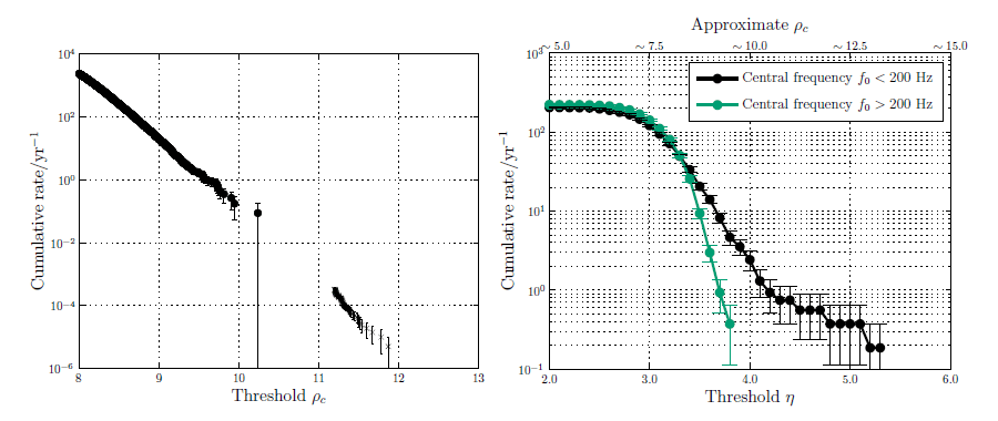

Figure 3: False alarm rate versus detection statistic for compact binary coalescence (CBC) and burst searches on 2009 – 2010 LIGO–Virgo data. Left: Cumulative rate of background events for a subset of the CBC search parameter space, as a function of the threshold ranking statistic  [19*]. Different methods were used to estimate the background for rate for high and low , which is why there is an apparent gap in the data points. The background for the full search was approximately a factor of six higher. Right: Cumulative rate of background events for the burst search, as a function of the coherent network amplitude  [14*]. For ease of comparison, we have also plotted the approximate equivalent for the burst search (an exact identification is not possible as the search methods differ). The burst events are divided into two sets based on their central frequency.

Figure 3* shows the noise background as a function of detection statistic for the low-mass binary coalescence and burst searches with the 2009 – 2010 LIGO–Virgo data [19*, 14*].² For binary mergers, the background rate decreases by a factor of  100 for every unit increase in combined SNR . Here is a combined, re-weighted SNR [29, 19]. The re-weighting is designed to reduce the SNR of glitches while leaving signals largely unaffected. Consequently, for a signal, is essentially the root-sum-square of the SNRs in the individual detectors. For bursts, we use the coherent network amplitude , which measures the degree of correlation between the detectors [22, 86]. Glitches have little correlated energy and so give low values of . Both and give an indication of the amplitude of the signal and can be used to rank events.

For CBC signals, we conservatively estimate that a threshold of 12 is required for a FAR below in aLIGO–AdV. To arrive at this estimate, we begin with Figure 3* which indicates that an SNR of around 10.5 corresponds to a FAR of . However, this corresponds to only a subspace of the CBC parameter space and the background of the full search is a factor of six higher. Additionally, due to the improved low frequency sensitivity of the advanced detectors and the inclusion of templates for binaries with (aligned) component spins, at least ten times as many waveform templates are required to perform the search [84, 34, 88, 46]. The background increases approximately linearly with the number of templates required. Consequently, we expect a background around a factor of 100 higher than indicated by Figure 3*, which leads us to quote a threshold of 12 for a FAR of  [31*]. A combined SNR of 12 corresponds to a single-detector SNR of 8.5 in each of two detectors, or 7 in each of three detectors.

Instrumental disturbances in the data can have a greater effect on the burst search. At frequencies above 200 Hz, the rate of background events falls off steeply as a function of amplitude. At lower frequencies, however, the data often exhibit a significant tail of loud background events that are not simply removed by multi-detector consistency tests. Although the advanced detectors are designed with many technical improvements, we anticipate that similar features will persist, particularly at low frequencies. Improvements to detection pipelines, which better distinguish between glitches and potential waveforms, can help eliminate these tails (e.g., [66]). For a given FAR, the detection threshold may need to be tuned for different frequency ranges; for the initial detectors, a threshold of – (approximately equivalent to from Figure 3*) was needed for a FAR of  [14*]. The unambiguous observation of an electromagnetic counterpart could increase the detection confidence.

3.2 Sky localization

Following the detection by the aLIGO–AdV network of a GW transient, determining the source’s location is a question for parameter estimation. Typically, posterior probability distributions for the sky position are constructed following a Bayesian framework [110*, 43*, 98*]. Information comes from the time of arrival, plus the phase and amplitude of the GW.

An intuitive understanding of localization can be gained by considering triangulation using the observed time delays between sites [55*, 56]. The effective single-site timing accuracy is approximately

where is the SNR in the given detector and is the effective bandwidth of the signal in the detector, typically of order 100 Hz. Thus a typical timing accuracy is on the order of (about 1/100 of the light travel time between sites). This sets the localization scale. The simple model of equation (1*) ignores many other relevant issues such as information from the signal amplitudes across the detector network, uncertainty in the emitted gravitational waveform, instrumental calibration accuracies, and correlation of sky location with other binary parameters  [55, 112, 111, 80, 109*, 79*, 99*, 31*, 98*]. While many of these affect the measurement of the time of arrival in individual detectors, such factors are largely common between two similar detectors, so the time difference between the two detectors is relatively uncorrelated with these nuisance parameters.

The triangulation approach underestimates how well a source can be localized, since it does not include all the relevant information. Its predictions can be improved by introducing the requirement of phase consistency between detectors [60*]. Triangulation always performs poorly for a two-detector network, but, with the inclusion of phase coherence, can provide an estimate for the average performance of a three-detector network [31*].³

Source localization using only timing for a two-site network yields an annulus on the sky; see Figure 4*. Additional information such as signal amplitude, spin, and precession effects resolve this to only parts of the annulus, but even then sources will only be localized to regions of hundreds to thousands of square degrees [99*, 31*]. An example of a two-detector BNS localization is shown in Figure 5*. The posterior probability distribution is primarily distributed along a ring, but this ring is broken, such that there are clear maxima.

Figure 4: Source localization by triangulation for the aLIGO–AdV network. The locations of the three detectors are indicated by black dots, with LIGO Hanford labeled H; LIGO Livingston as L, and Virgo as V. The locus of constant time delay (with associated timing uncertainty) between two detectors forms an annulus on the sky concentric about the baseline between the two sites (labeled by the two detectors). For three detectors, these annuli may intersect in two locations. 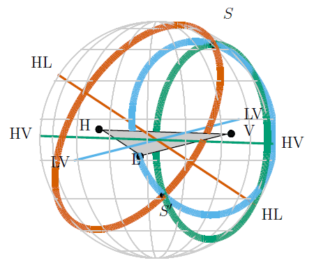One is centered on the true source direction (), while the other () is its mirror image with respect to the geometrical plane passing through the three sites. For four or more detectors there is a unique intersection region of all of the annuli. Figure adapted from [41].

Figure 5: Posterior probability density for sky location for an example binary neutron-star coalescence observed with a two-detector network. Left: Map produced by the low-latency bayestar code [99*, 98*]. Right: Map produced by the higher-latency (non-spinning) LALInference [110*], which also produces posterior estimates for other parameters. These algorithms are discussed in Section 3.2.1. The star indicates the true source location. 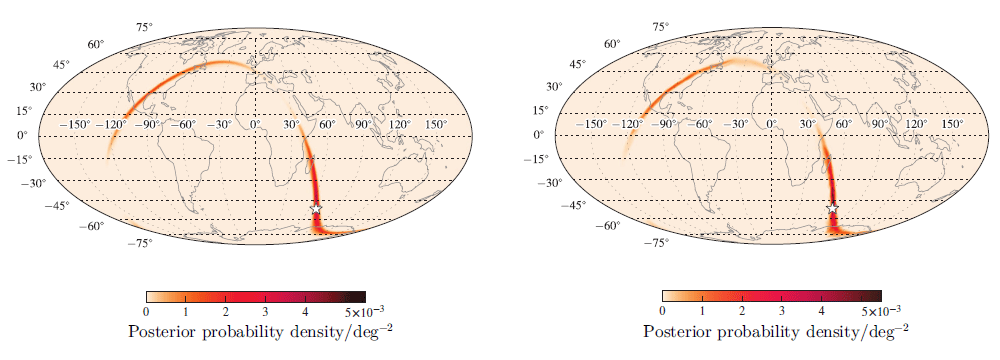The event has a network signal-to-noise ratio of using a noise curve appropriate for the first aLIGO run (O1, see Section 4.1). The plot is a Mollweide projection in geographic coordinates. Image reproduced with permission from [31*], copyright by APS; further mock sky maps for the first two observing runs can be found at www.ligo.org/scientists/first2years/ for binary neutron-star signals and www.ligo.org/scientists/burst-first2years/ for burst signals.

For three detectors, the time delays restrict the source to two sky regions which are mirror images with respect to the plane passing through the three sites. It is often possible to eliminate one of these regions by requiring consistent amplitudes in all detectors. For signals just above the detection threshold, this typically yields regions with areas of several tens to hundreds of square degrees. Additionally, for BNSs, it is often possible to obtain a reasonable estimate of the distance to the source [109*, 31*], which can be used to further aid electromagnetic observations [79*, 32]. If there is significant difference in sensitivity between detectors, the source is less well localized and we may be left with the majority of the annulus on the sky determined by the two most sensitive detectors. With four or more detectors, timing information alone is sufficient to localize to a single sky region, and the additional baselines help to limit the region to under for some signals.

From Eq. (1*), it follows that the linear size of the localization ellipse scales inversely with the SNR of the signal and the frequency bandwidth of the signal in the detector [31*]. For GWs that sweep across the band of the detector, such as CBC signals, the effective bandwidth is  100 Hz, determined by the most sensitive frequencies of the detector. For shorter transients the bandwidth depends on the specific signal. For example, GWs emitted by various processes in core-collapse supernovae are anticipated to have relatively large bandwidths, between 150 – 500 Hz [48, 82, 113, 83], largely independent of detector configuration. By contrast, the sky localization region for narrowband burst signals may consist of multiple disconnected regions and exhibit fringing features; see for example [72, 16*, 51*].

Some GW searches are triggered by electromagnetic observations, and in these cases localization information is known a priori. For example, in GW searches triggered by gamma-ray bursts [18*, 7, 6] the triggering space-based telescope provides the localization. The detection of a GW transient associated with a gamma-ray burst would provide strong evidence for the burst progenitor; for example, BNS mergers are considered the likely progenitors of most short gamma-ray bursts. It is therefore important to have high-energy telescopes operating during the advanced-detector era. Furthermore, the rapid identification of a GW counterpart to such a trigger could prompt further spectroscopic studies and longer, deeper follow-up in different wavelengths that may not always be done in response to gamma-ray bursts. This is particularly important for gamma-ray bursts with larger sky localization uncertainties, such as those reported by the Fermi GBM, which are not followed up as frequently as bursts reported by Swift.

Finally, all GW data are stored permanently, so that it is possible to perform retroactive analyses at any time.

3.2.1 Localization of binary neutron stars

Providing prompt localizations for GW signals helps to maximise the chance that electromagnetic observatories can catch a counterpart. Sky maps will be produced at several different latencies, with updates coming from more computationally expensive algorithms that refine our understanding of the source. For BNS signals, rapid sky localization is performed using bayestar [98*], a Bayesian parameter-estimation code that computes source location using output from the detection pipeline. It can produce sky maps (as in Figure 5*) with latencies of only a few seconds. A similar approach to low-latency localization has been separately developed by [42], who find results consistent with bayestar.

At higher latency, CBC parameter estimation is performed using the stochastic sampling algorithms of LALInference [110*]. LALInference constructs posterior probability distributions for system parameters (not just location, but also mass, orientation, etc. [3]) by matching GW templates to the detector strain [44, 65]. Computing these waveforms is computationally expensive; this expense increases as the detectors’ low-frequency sensitivity improves and waveforms must be computed down to lower frequencies. The quickest LALInference BNS follow-up is computed using waveforms that do not include the full effects of component spin [99*, 31*], sky locations can then be reported with latency of hours to a couple of days. Parameter estimation is then performed using more accurate waveform approximates (those that include the full effects of spin precession), which can take weeks or months [57*]. Methods of reducing the computational cost are actively being investigated (e.g., [37, 89, 36]).

There is negligible difference between the low-latency bayestar and the mid-latency non-spinning LALInference analyses if the BNS signal is loud enough to produce a trigger in all detectors: if there is not, LALInference currently gives a more precise localization, as it still uses information from the non-triggered detector [99*, 98*]. It is hoped to improve bayestar localization in the future by including information about sub-threshold signals. Provided that BNSs are slowly spinning [77], there should be negligible difference between the mid-latency non-spinning LALInference and the high-latency fully spinning LALInference analyses [57].

Results from an astrophysically motivated population of BNS signals, assuming a detection threshold of a SNR of 12, are shown in Figure 6* [99*, 31*]. Sky localization is measured by the 90% credible region , the smallest area enclosing 90% of the total posterior probability, and the searched area , the area of the smallest credible region that encompasses the true position [97]: gives the area of the sky that must be covered to expect a 90% chance of including the source location, and gives the area that would be viewed before the true location using the given sky map. Results from both the low-latency bayestar and mid-latency non-spinning LALInference analyses are shown. These are discussed further in Section 4.1 and Section 4.2. The two-detector localizations get slightly worse going from O1 to O2. This is because although the detectors improve in sensitivity at every frequency, with the assumed noise curves the BNS signal bandwidth is lower in O2 for a given SNR because of enhanced sensitivity at low frequencies [99*]. Despite this, the overall sky-localization in O2 is better than in O1. As sky localization improves with the development of the detector network [96*, 72, 109*, 91*], these results mark the baseline of performance for the advanced-detector era.

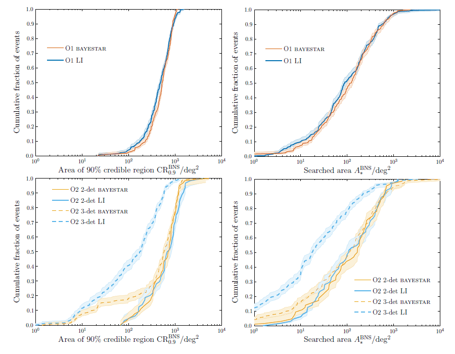
Figure 6: Anticipated binary neutron-star sky localization during the first two observing runs (top: O1, see Section 4.1; bottom: O2, see Section 4.2). The plots show the cumulative fractions of events with sky-localization areas smaller than the abscissa value. Left: Sky area of 90% credible region , the (smallest) area enclosing 90% of the total posterior probability. Right: Searched area , the area of the smallest credible region containing the true position. Results are shown for the low-latency bayestar [98] and higher-latency (non-spinning) LALInference (LI) [110*] codes. The O2 results are divided into those where two detectors (2-det) are operating in coincidence, and those where three detectors (3-det) are operating: assuming a duty cycle of  80% for each instrument, the two-detector network would be operating for  40% of the total time and the three-detector network  50% of the time. The shaded areas indicate the 68% confidence intervals on the cumulative distributions. A detection threshold of a signal-to-noise ratio of 12 is used and results are taken from [31*, 99*].

3.2.2 Localization of bursts

The lowest latency burst sky maps are produced as part of the coherent WaveBurst (cWB) [71*, 73*] detection pipeline, earlier versions of which were used in prior burst searches [12, 14*, 70*]. Sky maps are produced using a constrained likelihood algorithm that coherently combines data from all the detectors; unlike other approaches, this is not fully Bayesian. The resulting sky maps currently show calibration issues.⁴ The confidence is over-estimated at low levels and under-estimated at high levels. However, the searched areas are consistent with those from other burst techniques, indicating that cWB maps can be used to guide observations. The cWB sky maps calculated with a latency of a few minutes; following detection, further parameter-estimation codes analyze the data.

At higher latency, burst signals are analyzed by LALInferenceBurst (LIB), a stochastic sampling algorithm similar to the LALInference code used to reconstruct CBC signals [110*], and BayesWave, a reversible jump Markov-chain Monte Carlo algorithm that models both signals and glitches [43]. LIB uses a sine–Gaussian waveform (in place of the CBC templates used by LALInference), and can produce sky maps in a few hours. BayesWave uses a variable number of sine–Gaussian wavelets to model a signal and glitches while also fitting for the noise spectrum using BayesLine [75]; it produces sky maps with a latency of a few days. Sky maps produced by LIB and BayesWave should be similar, with performance depending upon the actual waveform.

A full study of burst localization in the first two years of the aLIGO–AdV network was completed in [51*]. This study was conducted using cWB and LIB. Sky localization was quantified by the searched area. Using an approximate FAR threshold of , the median localization was shown to be – for a two-detector network in 2015 – 2016 and – for a three-detector network in 2016 – 2017, with the localization and relative performance of the algorithms depending upon the waveform morphology. Results for Gaussian, sine–Gaussian, broadband white-noise and BBH waveforms are shown in Figure 7* (for the two-detector O1 network and the three-detector O2 network, cf. Figure 6*). The largest difference between the codes here is for the white-noise bursts; for a three-detector network, LIB achieves better localization than cWB for Gaussian and sine–Gaussian bursts. The variety of waveform morphologies reflect the range of waveforms that could be detected in a burst search [16].

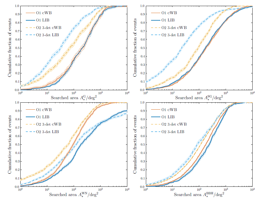
Figure 7: Simulated sky localization for Gaussian (G; top left), sine–Gaussian (SG; top right), broadband white-noise (WN; bottom left) and binary black-hole (BBH; bottom right) bursts during the first two observing runs (O1, see Section 4.1, and O2, see Section 4.2). The plots show the cumulative fractions of events with searched areas smaller than the abscissa value. Results are shown for the low-latency coherent WaveBurst (cWB) [70, 71, 73] and higher-latency LALInferenceBurst (LIB) [110*] codes. The O2 results consider only a three-detector (3-det) network; assuming an instrument duty cycle of  80%, this would be operational  50% of the time. The shaded areas indicate the 68% confidence intervals on the cumulative distributions. A detection threshold of a false alarm rate of approximately is used and results are taken from [51*].