A point particle carries a scalar charge ![]() and moves on a world line
and moves on a world line ![]() described by relations
described by relations
![]() , in which
, in which ![]() is an arbitrary parameter. The particle generates a scalar potential
is an arbitrary parameter. The particle generates a scalar potential ![]() and a field
and a field ![]() . The dynamics of the entire system is governed by the action
. The dynamics of the entire system is governed by the action
The field action is given by
where the integration is over all of spacetime; the field is coupled to the Ricci scalar Demanding that the total action be stationary under a variation ![]() of the field configuration yields
the wave equation
of the field configuration yields
the wave equation
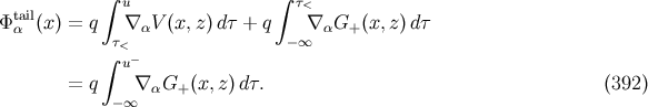
The retarded solution to Equation (385![]() ) is
) is ![]() , where
, where ![]() is the
retarded Green’s function introduced in Section 4.3. After substitution of Equation (386
is the
retarded Green’s function introduced in Section 4.3. After substitution of Equation (386![]() ) we obtain
) we obtain
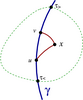
We now specialize Equation (389![]() ) to a point
) to a point ![]() near the world line (see Figure 9
near the world line (see Figure 9![]() ). We let
). We let ![]() be
the normal convex neighbourhood of this point, and we assume that the world line traverses
be
the normal convex neighbourhood of this point, and we assume that the world line traverses ![]() . Let
. Let
![]() be the value of the proper-time parameter at which
be the value of the proper-time parameter at which ![]() enters
enters ![]() from the past, and let
from the past, and let ![]() be
its value when the world line leaves
be
its value when the world line leaves ![]() . Then Equation (389
. Then Equation (389![]() ) can be broken down into the three
integrals
) can be broken down into the three
integrals
The third integration vanishes because ![]() is then in the past of
is then in the past of ![]() , and
, and ![]() . For the second
integration,
. For the second
integration, ![]() is the normal convex neighbourhood of
is the normal convex neighbourhood of ![]() , and the retarded Green’s function can be
expressed in the Hadamard form produced in Section 4.3.2. This gives
, and the retarded Green’s function can be
expressed in the Hadamard form produced in Section 4.3.2. This gives
and to evaluate this we refer back to Section 3.3 and let ![]() be the retarded point
associated with
be the retarded point
associated with ![]() ; these points are related by
; these points are related by ![]() and
and ![]() is the retarded
distance between
is the retarded
distance between ![]() and the world line. We resume the index convention of Section 3.3: To
tensors at
and the world line. We resume the index convention of Section 3.3: To
tensors at ![]() we assign indices
we assign indices ![]() ,
, ![]() , etc.; to tensors at
, etc.; to tensors at ![]() we assign indices
we assign indices ![]() ,
, ![]() ,
etc.; and to tensors at a generic point
,
etc.; and to tensors at a generic point ![]() on the world line we assign indices
on the world line we assign indices ![]() ,
, ![]() ,
etc.
,
etc.
To perform the first integration we change variables from ![]() to
to ![]() , noticing that
, noticing that ![]() increases as
increases as ![]() passes through
passes through ![]() . The change of
. The change of ![]() on the world line is given by
on the world line is given by
![]() , and we find that the first integral evaluates to
, and we find that the first integral evaluates to ![]() with
with ![]() identified with
identified with ![]() . The second integration is cut off at
. The second integration is cut off at ![]() by the step function, and we
obtain our final expression for the retarded potential of a point scalar charge:
by the step function, and we
obtain our final expression for the retarded potential of a point scalar charge:
When we differentiate the potential of Equation (390![]() ) we must keep in mind that a variation in
) we must keep in mind that a variation in ![]() induces
a variation in
induces
a variation in ![]() because the new points
because the new points ![]() and
and ![]() must also be linked by a null geodesic –
you may refer back to Section 3.3.2 for a detailed discussion. This means, for example, that the total
variation of
must also be linked by a null geodesic –
you may refer back to Section 3.3.2 for a detailed discussion. This means, for example, that the total
variation of ![]() is
is ![]() . The gradient of the
scalar potential is therefore given by
. The gradient of the
scalar potential is therefore given by
We shall now expand ![]() in powers of
in powers of ![]() , and express the results in terms of the
retarded coordinates
, and express the results in terms of the
retarded coordinates ![]() introduced in Section 3.3. It will be convenient to decompose
introduced in Section 3.3. It will be convenient to decompose
![]() in the tetrad
in the tetrad ![]() that is obtained by parallel transport of
that is obtained by parallel transport of ![]() on the
null geodesic that links
on the
null geodesic that links ![]() to
to ![]() ; this construction is detailed in Section 3.3. Note
that throughout this section we set
; this construction is detailed in Section 3.3. Note
that throughout this section we set ![]() , where
, where ![]() is the rotation tensor defined by
Equation (138
is the rotation tensor defined by
Equation (138![]() ): The tetrad vectors
): The tetrad vectors ![]() are taken to be Fermi–Walker transported on
are taken to be Fermi–Walker transported on ![]() . The
expansion relies on Equation (166
. The
expansion relies on Equation (166![]() ) for
) for ![]() , Equation (168
, Equation (168![]() ) for
) for ![]() , and we shall need
, and we shall need
are frame components of the Ricci tensor evaluated at ![]() . We shall also need the expansions
. We shall also need the expansions
Collecting all these results gives
where
are frame components of the Riemann tensor evaluated at ![]() , and
, and
The gradient of the scalar potential can also be expressed in the Fermi normal coordinates of Section 3.2.
To effect this translation we make ![]() the new reference point on the world line. We
resume here the notation of Section 3.4 and assign indices
the new reference point on the world line. We
resume here the notation of Section 3.4 and assign indices ![]() ,
, ![]() , …to tensors at
, …to tensors at ![]() . The
Fermi normal coordinates are denoted
. The
Fermi normal coordinates are denoted ![]() , and we let
, and we let ![]() be the tetrad at
be the tetrad at ![]() that is obtained by parallel transport of
that is obtained by parallel transport of ![]() on the spacelike geodesic that links
on the spacelike geodesic that links ![]() to
to
![]() .
.
Our first task is to decompose ![]() in the tetrad
in the tetrad ![]() , thereby defining
, thereby defining ![]() and
and
![]() . For this purpose we use Equations (224
. For this purpose we use Equations (224![]() , 225
, 225![]() ) and (397
) and (397![]() , 398
, 398![]() ) to obtain
) to obtain
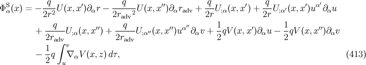
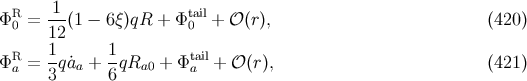
![[ ] [ 2] ( b) a 1 2 a 1 2 a b 3 Φ¯0 = 1 + 𝒪 (r ) Φ0 + r 1 − abΩ a + 2-r ˙a + 2r R 0b0Ω + 𝒪 (r ) Φa = − 1qa˙Ωa + -1(1 − 6ξ)qR + ¯Φtail+ 𝒪 (r) 2 a 12 0](article2722x.gif)
![[ ] b 1 2 b 1 2 b c 3 [ 2 ] ¯Φa = δ a + -r a aa − -r R a0cΩ + 𝒪 (r ) Φb + raa + 𝒪 (r ) Φ0 2 2 = − q-Ω − q-a ΩbΩ + 1qa Ωba − 1qR ΩbΩc Ω − 1-qR Ωb − 1qR Ωb Ωc r2 a r b a 2 b a 3 b0c0 a 6 a0b0 3 ab0c 1 [ b c ] 1 ( b) tail + 12-q R00 − Rbc Ω Ω − (1 − 6ξ)R Ωa + 6q Ra0 + RabΩ + Φ¯a + 𝒪 (r),](article2723x.gif)
We must still translate these results into the Fermi normal coordinates ![]() . For this we involve
Equations (221
. For this we involve
Equations (221![]() , 222
, 222![]() , 223
, 223![]() ), from which we deduce, for example,
), from which we deduce, for example,
in which all frame components (on the right-hand side of these relations) are now evaluated at ![]() ; to
obtain the second relation we expressed
; to
obtain the second relation we expressed ![]() as
as ![]() , since according to
Equation (221
, since according to
Equation (221![]() ),
), ![]() .
.
Collecting these results yields
In these expressions,
are frame components of the Ricci tensor, and ![]() is the Ricci scalar evaluated at
is the Ricci scalar evaluated at ![]() . Finally, we have
that
. Finally, we have
that
We shall now compute the averages of ![]() and
and ![]() over
over ![]() , a two-surface of constant
, a two-surface of constant
![]() and
and ![]() ; these will represent the mean value of the field at a fixed proper distance away
from the world line, as measured in a reference frame that is momentarily comoving with the
particle. The two-surface is charted by angles
; these will represent the mean value of the field at a fixed proper distance away
from the world line, as measured in a reference frame that is momentarily comoving with the
particle. The two-surface is charted by angles ![]() (
(![]() ) and it is described, in the
Fermi normal coordinates, by the parametric relations
) and it is described, in the
Fermi normal coordinates, by the parametric relations ![]() ; a canonical choice of
parameterization is
; a canonical choice of
parameterization is ![]() . Introducing the transformation matrices
. Introducing the transformation matrices
![]() , we find from Equation (127
, we find from Equation (127![]() ) that the induced metric on
) that the induced metric on ![]() is given by
is given by
The averaged fields are defined by
where the quantities to be integrated are scalar functions of the Fermi normal coordinates. The results are easy to establish, and we obtain The averaged field is still singular on the world line. Regardless, we shall take the formal limit
The singular potential
is the (unphysical) solution to Equations (385 To evaluate the integral of Equation (411![]() ) we assume once more that
) we assume once more that ![]() is sufficiently close to
is sufficiently close to ![]() that the world line traverses
that the world line traverses ![]() (refer back to Figure 9
(refer back to Figure 9![]() ). As before we let
). As before we let ![]() and
and ![]() be the values
of the proper-time parameter at which
be the values
of the proper-time parameter at which ![]() enters and leaves
enters and leaves ![]() , respectively. Then Equation (411
, respectively. Then Equation (411![]() )
can be broken down into the three integrals,
)
can be broken down into the three integrals,
The first integration vanishes because ![]() is then in the chronological future of
is then in the chronological future of ![]() , and
, and ![]() by Equation (286
by Equation (286![]() ). Similarly, the third integration vanishes because
). Similarly, the third integration vanishes because ![]() is then in the chronological past of
is then in the chronological past of
![]() . For the second integration,
. For the second integration, ![]() is the normal convex neighbourhood of
is the normal convex neighbourhood of ![]() , the
singular Green’s function can be expressed in the Hadamard form of Equation (297
, the
singular Green’s function can be expressed in the Hadamard form of Equation (297![]() ), and we
have
), and we
have
To evaluate these we re-introduce the retarded point ![]() and let
and let ![]() be the
advanced point associated with
be the
advanced point associated with ![]() ; we recall from Section 3.4.4 that these points are related by
; we recall from Section 3.4.4 that these points are related by
![]() and that
and that ![]() is the advanced distance between
is the advanced distance between ![]() and the world
line.
and the world
line.
To perform the first integration we change variables from ![]() to
to ![]() , noticing that
, noticing that ![]() increases as
increases as
![]() passes through
passes through ![]() ; the integral evaluates to
; the integral evaluates to ![]() . We do the same for the second
integration, but we notice now that
. We do the same for the second
integration, but we notice now that ![]() decreases as
decreases as ![]() passes through
passes through ![]() ; the integral evaluates to
; the integral evaluates to
![]() . The third integration is restricted to the interval
. The third integration is restricted to the interval ![]() by the step
function, and we obtain our final expression for the singular potential of a point scalar charge:
by the step
function, and we obtain our final expression for the singular potential of a point scalar charge:
We use the techniques of Section 5.1.3 to differentiate the potential of Equation (412![]() ). We find
). We find
We recall first that a relation between retarded and advanced times was worked out in Equation (229![]() ),
that an expression for the advanced distance was displayed in Equation (230
),
that an expression for the advanced distance was displayed in Equation (230![]() ), and that Equations (231
), and that Equations (231![]() )
and (232
)
and (232![]() ) give expansions for
) give expansions for ![]() and
and ![]() , respectively.
, respectively.
To derive an expansion for ![]() we follow the general method of Section 3.4.4 and define a
function
we follow the general method of Section 3.4.4 and define a
function ![]() of the proper-time parameter on
of the proper-time parameter on ![]() . We have that
. We have that
where overdots indicate differentiation with respect to ![]() , and where
, and where ![]() . The leading term
. The leading term
![]() was worked out in Equation (393
was worked out in Equation (393![]() ), and the derivatives of
), and the derivatives of ![]() are given
by
are given
by
and
according to Equations (395![]() ) and (276
) and (276![]() ). Combining these results together with Equation (229
). Combining these results together with Equation (229![]() ) for
) for ![]() gives
gives
We proceed similarly to derive an expansion for ![]() . Here we introduce the functions
. Here we introduce the functions
![]() and express
and express ![]() as
as ![]() . The leading term
. The leading term
![]() was computed in Equation (394
was computed in Equation (394![]() ), and
), and
follows from Equation (276![]() ). Combining these results together with Equation (229
). Combining these results together with Equation (229![]() ) for
) for ![]() gives
gives
The last expansion we shall need is
which follows at once from Equation (396 It is now a straightforward (but tedious) matter to substitute these expansions (all of them!) into
Equation (413![]() ) and obtain the projections of the singular field
) and obtain the projections of the singular field ![]() in the same tetrad
in the same tetrad ![]() that
was employed in Section 5.1.3. This gives
that
was employed in Section 5.1.3. This gives
The difference between the retarded field of Equations (397![]() , 398
, 398![]() ) and the singular field of
Equations (418
) and the singular field of
Equations (418![]() , 419
, 419![]() ) defines the radiative field
) defines the radiative field ![]() . Its tetrad components are
. Its tetrad components are
The retarded field ![]() of a point scalar charge is singular on the world line, and this behaviour makes
it difficult to understand how the field is supposed to act on the particle and affect its motion. The field’s
singularity structure was analyzed in Sections 5.1.3 and 5.1.4, and in Section 5.1.5 it was shown to
originate from the singular field
of a point scalar charge is singular on the world line, and this behaviour makes
it difficult to understand how the field is supposed to act on the particle and affect its motion. The field’s
singularity structure was analyzed in Sections 5.1.3 and 5.1.4, and in Section 5.1.5 it was shown to
originate from the singular field ![]() ; the radiative field
; the radiative field ![]() was then shown to
be smooth on the world line.
was then shown to
be smooth on the world line.
To make sense of the retarded field’s action on the particle we temporarily model the scalar charge not
as a point particle, but as a small hollow shell that appears spherical when observed in a reference frame
that is momentarily comoving with the particle; the shell’s radius is ![]() in Fermi normal coordinates, and
it is independent of the angles contained in the unit vector
in Fermi normal coordinates, and
it is independent of the angles contained in the unit vector ![]() . The net force acting at proper time
. The net force acting at proper time ![]() on
this hollow shell is the average of
on
this hollow shell is the average of ![]() over the surface of the shell. This was worked out at
the end of Section 5.1.4, and ignoring terms that disappear in the limit
over the surface of the shell. This was worked out at
the end of Section 5.1.4, and ignoring terms that disappear in the limit ![]() , we obtain
, we obtain
Substituting Equations (424![]() ) and (426
) and (426![]() ) into Equation (387
) into Equation (387![]() ) gives rise to the equations of motion
) gives rise to the equations of motion
Apart from the term proportional to ![]() , the averaged field of Equation (424
, the averaged field of Equation (424![]() ) has exactly the same
form as the radiative field of Equation (422
) has exactly the same
form as the radiative field of Equation (422![]() ), which we re-express as
), which we re-express as
The equations of motion displayed in Equations (427![]() ) and (428
) and (428![]() ) are third-order differential equations
for the functions
) are third-order differential equations
for the functions ![]() . It is well known that such a system of equations admits many unphysical
solutions, such as runaway situations in which the particle’s acceleration increases exponentially with
. It is well known that such a system of equations admits many unphysical
solutions, such as runaway situations in which the particle’s acceleration increases exponentially with ![]() ,
even in the absence of any external force [25
,
even in the absence of any external force [25![]() , 30, 47
, 30, 47![]() ]. And indeed, our equations of motion do not yet
incorporate an external force which presumably is mostly responsible for the particle’s acceleration. Both
defects can be cured in one stroke. We shall take the point of view, the only admissible one in a classical
treatment, that a point particle is merely an idealization for an extended object whose internal
structure – the details of its charge distribution – can be considered to be irrelevant. This view
automatically implies that our equations are meant to provide only an approximate description of the
object’s motion. It can then be shown [47, 26] that within the context of this approximation, it
is consistent to replace, on the right-hand side of the equations of motion, any occurrence of
the acceleration vector by
]. And indeed, our equations of motion do not yet
incorporate an external force which presumably is mostly responsible for the particle’s acceleration. Both
defects can be cured in one stroke. We shall take the point of view, the only admissible one in a classical
treatment, that a point particle is merely an idealization for an extended object whose internal
structure – the details of its charge distribution – can be considered to be irrelevant. This view
automatically implies that our equations are meant to provide only an approximate description of the
object’s motion. It can then be shown [47, 26] that within the context of this approximation, it
is consistent to replace, on the right-hand side of the equations of motion, any occurrence of
the acceleration vector by ![]() , where
, where ![]() is the external force acting on the particle.
Because
is the external force acting on the particle.
Because ![]() is a prescribed quantity, differentiation of the external force does not produce
higher derivatives of the functions
is a prescribed quantity, differentiation of the external force does not produce
higher derivatives of the functions ![]() , and the equations of motion are properly of second
order.
, and the equations of motion are properly of second
order.
We shall therefore write, in the final analysis, the equations of motion in the form
and where| http://www.livingreviews.org/lrr-2004-6 |
© Max Planck Society
Problems/comments to |
![Φ (u, r,Ωa ) ≡ Φ (x)eα(x) 0 α 0 = qaa Ωa + 1qRa0b0 ΩaΩb + -1-(1 − 6ξ) qR + Φtail+ 𝒪 (r), (397 ) r 2 12 0 Φa(u, r,Ωa ) ≡ Φ α(x)eαa(x) q q 1 1 ( ) = − -2Ωa − -abΩbΩa − -qRb0c0Ωb ΩcΩa − -q Ra0b0Ωb − Rab0cΩbΩc r [ r 3 ] 6 ( ) + 1-q R00 − RbcΩbΩc − (1 − 6ξ)R Ωa + 1q Ra0 + RabΩb + Φtail+ 𝒪 (r), (398 ) 12 6 a](article2697x.gif)
![Φ¯ (t,s,ωa) ≡ Φ (x)¯eα(x) 0 α 0 = − 1qa˙ ωa + -1(1 − 6ξ)qR + ¯Φtail+ 𝒪 (s ), (400 ) 2 a 12 0 Φ¯a (t,s,ωa) ≡ Φ α(x)¯eαa(x) q q ( ) 3 3 ( ) 1 1 = − --ωa − ---aa − abωb ωa + -qabωbaa − -q abωb 2ωa + -q˙a0ωa + --q˙aa s2 2s 4 8 8 3 − 1qR ωb + 1-qR ωbωcω + -1-q[R − R ωbωc − (1 − 6ξ)R ]ω 3 a0b0 6 b0c0 a 12 00 bc a 1 ( b) tail + 6q Ra0 + Rabω + ¯Φ a + 𝒪 (s). (401 )](article2735x.gif)
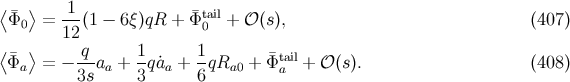
![S a S α Φ0(u, r,Ω ) ≡ Φ α(x)e0(x) q- a 1- a b = r aaΩ + 2 qRa0b0Ω Ω + 𝒪 (r), (418 ) ΦS(u, r,Ωa) ≡ ΦS (x)eα(x) a α a = − q-Ω − qa Ωb Ω − 1q ˙a − 1qR ΩbΩc Ω − 1-q(R Ωb − R Ωb Ωc) r2 a r b a 3 a 3 b0c0 a 6 a0b0 ab0c 1-- [ b c ] 1- b + 12q R00 − RbcΩ Ω − (1 − 6ξ )R Ωa + 6qRab Ω , (419 )](article2853x.gif)
![[ ] 1 1 ∫ τ− (m + δm )a μ = q2(δμν + u μuν) -˙aν + --Rνλuλ + ∇ νG+ (z(τ),z(τ′)) dτ′ (427 ) 3 6 − ∞](article2878x.gif)
![[ ∫ − ] Du-μ- μ 2 μ μ -1-Df-νext 1- ν λ τ ν ′ ′ m dτ = fext + q (δν + u u ν) 3m dτ + 6R λu + ∇ G+ (z (τ ),z(τ)) dτ (431 ) −∞](article2895x.gif)