The derivation of the MiSaTaQuWa equations of motion presented in Section 5.3 was framed within the
paradigm introduced in Sections 5.1 and 5.2 to describe the motion of a point scalar charge, and a point
electric charge, respectively. While this paradigm is well suited to fields that satisfy linear wave equations, it
is not the best conceptual starting point in the nonlinear context of general relativity. The linearization of
the Einstein field equations with respect to the small parameter ![]() did allow us to use the same
mathematical techniques as in Sections 5.1 and 5.2, but the validity of the perturbative method must
be critically examined when the gravitational potentials are allowed to be singular. So while
Equation (550
did allow us to use the same
mathematical techniques as in Sections 5.1 and 5.2, but the validity of the perturbative method must
be critically examined when the gravitational potentials are allowed to be singular. So while
Equation (550![]() ) does indeed give the correct equations of motion when
) does indeed give the correct equations of motion when ![]() is small, its previous
derivation leaves much to be desired. In this section I provide another derivation that is entirely free
of conceptual and technical pitfalls. Here the point mass will be replaced by a nonrotating
black hole, and the perturbation’s singular behaviour on the world line will be replaced by a
well-behaved metric at the event horizon. We will use the powerful technique of matched asymptotic
expansions [35, 32, 58
is small, its previous
derivation leaves much to be desired. In this section I provide another derivation that is entirely free
of conceptual and technical pitfalls. Here the point mass will be replaced by a nonrotating
black hole, and the perturbation’s singular behaviour on the world line will be replaced by a
well-behaved metric at the event horizon. We will use the powerful technique of matched asymptotic
expansions [35, 32, 58![]() , 19, 1, 20].
, 19, 1, 20].
The problem presents itself with a clean separation of length scales, and the method relies entirely on
this. On the one hand we have the length scale associated with the small black hole, which is set by its mass
![]() . On the other hand we have the length scale associated with the background spacetime in which the
black hole moves, which is set by the radius of curvature
. On the other hand we have the length scale associated with the background spacetime in which the
black hole moves, which is set by the radius of curvature ![]() ; formally this is defined so that a typical
component of the background spacetime’s Riemann tensor is equal to
; formally this is defined so that a typical
component of the background spacetime’s Riemann tensor is equal to ![]() up to a numerical
factor of order unity. We demand that
up to a numerical
factor of order unity. We demand that ![]() . As before we assume that the background
spacetime contains no matter, so that its metric is a solution to the Einstein field equations in
vacuum.
. As before we assume that the background
spacetime contains no matter, so that its metric is a solution to the Einstein field equations in
vacuum.
For example, suppose that our small black hole of mass ![]() is on an orbit of radius
is on an orbit of radius ![]() around another
black hole of mass
around another
black hole of mass ![]() . Then
. Then ![]() and we take
and we take ![]() to be much smaller than the orbital
separation. Notice that the time scale over which the background geometry changes is of the order of the
orbital period
to be much smaller than the orbital
separation. Notice that the time scale over which the background geometry changes is of the order of the
orbital period ![]() , so that this does not constitute a separate scale. Similarly, the inhomogeneity
scale – the length scale over which the Riemann tensor of the background spacetime changes – is of
order
, so that this does not constitute a separate scale. Similarly, the inhomogeneity
scale – the length scale over which the Riemann tensor of the background spacetime changes – is of
order ![]() and also does not constitute an independent scale. (In this discussion
we have considered
and also does not constitute an independent scale. (In this discussion
we have considered ![]() to be of order unity, so as to represent a strong-field, fast-motion
situation.)
to be of order unity, so as to represent a strong-field, fast-motion
situation.)
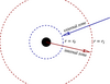
Let ![]() be a meaningful measure of distance from the small black hole, and let us consider a region of
spacetime defined by
be a meaningful measure of distance from the small black hole, and let us consider a region of
spacetime defined by ![]() , where
, where ![]() is a constant that is much smaller than
is a constant that is much smaller than ![]() . This inequality
defines a narrow world tube that surrounds the small black hole, and we shall call this region the internal
zone (see Figure 10
. This inequality
defines a narrow world tube that surrounds the small black hole, and we shall call this region the internal
zone (see Figure 10![]() ). In the internal zone the gravitational field is dominated by the black hole, and the
metric can be expressed as
). In the internal zone the gravitational field is dominated by the black hole, and the
metric can be expressed as
Consider now a region of spacetime defined by ![]() , where
, where ![]() is a constant that is much larger
than
is a constant that is much larger
than ![]() ; this region will be called the external zone (see Figure 10
; this region will be called the external zone (see Figure 10![]() ). In the external zone the gravitational
field is dominated by the conditions in the external universe, and the metric can be expressed as
). In the external zone the gravitational
field is dominated by the conditions in the external universe, and the metric can be expressed as
The metric ![]() returned by the procedure described in the preceding paragraph is a
functional of a world line
returned by the procedure described in the preceding paragraph is a
functional of a world line ![]() that represents the motion of the small black hole in the background
spacetime. Our goal is to obtain a description of this world line, in the form of equations of motion to be
satisfied by the black hole; these equations will be formulated in the background spacetime. It is important
to understand that fundamentally,
that represents the motion of the small black hole in the background
spacetime. Our goal is to obtain a description of this world line, in the form of equations of motion to be
satisfied by the black hole; these equations will be formulated in the background spacetime. It is important
to understand that fundamentally, ![]() exists only as an external-zone construct: It is only in the external
zone that the black hole can be thought of as moving on a world line; in the internal zone the black hole is
revealed as an extended object and the notion of a world line describing its motion is no longer
meaningful.
exists only as an external-zone construct: It is only in the external
zone that the black hole can be thought of as moving on a world line; in the internal zone the black hole is
revealed as an extended object and the notion of a world line describing its motion is no longer
meaningful.
Equations (555![]() ) and (556
) and (556![]() ) give two different expressions for the metric of the same spacetime; the
first is valid in the internal zone
) give two different expressions for the metric of the same spacetime; the
first is valid in the internal zone ![]() , while the second is valid in the external zone
, while the second is valid in the external zone
![]() . The fact that
. The fact that ![]() allows us to define a buffer zone in which
allows us to define a buffer zone in which ![]() is restricted to
the interval
is restricted to
the interval ![]() . In the buffer zone
. In the buffer zone ![]() is simultaneously much larger than
is simultaneously much larger than ![]() and
much smaller than
and
much smaller than ![]() – a typical value might be
– a typical value might be ![]() – and Equations (555
– and Equations (555![]() , 556
, 556![]() ) are
simultaneously valid. Since the two metrics are the same up to a diffeomorphism, these expressions must
agree. And since
) are
simultaneously valid. Since the two metrics are the same up to a diffeomorphism, these expressions must
agree. And since ![]() is a functional of a world line
is a functional of a world line ![]() while
while ![]() contains no such information, matching the metrics necessarily determines the motion of the small
black hole in the background spacetime. What we have here is a beautiful implementation of the
general observation that the motion of self-gravitating bodies is determined by the Einstein field
equations.
contains no such information, matching the metrics necessarily determines the motion of the small
black hole in the background spacetime. What we have here is a beautiful implementation of the
general observation that the motion of self-gravitating bodies is determined by the Einstein field
equations.
It is not difficult to recognize that the metrics of Equations (555![]() , 556
, 556![]() ) can be matched in the buffer
zone. When
) can be matched in the buffer
zone. When ![]() in the internal zone, the metric of the unperturbed black hole can be
expanded as
in the internal zone, the metric of the unperturbed black hole can be
expanded as ![]() , where
, where ![]() is the metric of flat spacetime (in
asymptotically inertial coordinates) and the symbol
is the metric of flat spacetime (in
asymptotically inertial coordinates) and the symbol ![]() means “and a term of the form…”. On the other
hand, dimensional analysis dictates that
means “and a term of the form…”. On the other
hand, dimensional analysis dictates that ![]() be of the form
be of the form ![]() while
while ![]() should be expressed as
should be expressed as ![]() . Altogether we obtain
. Altogether we obtain
Matching the metrics of Equations (555![]() ) and (556
) and (556![]() ) in the buffer zone can be carried out in practice
only after performing a transformation from the external coordinates used to express
) in the buffer zone can be carried out in practice
only after performing a transformation from the external coordinates used to express ![]() to
the internal coordinates employed for
to
the internal coordinates employed for ![]() . The details of this coordinate transformation will
be described in Section 5.4.4, and the end result of matching – the MiSaTaQuWa equations of motion – will
be revealed in Section 5.4.5.
. The details of this coordinate transformation will
be described in Section 5.4.4, and the end result of matching – the MiSaTaQuWa equations of motion – will
be revealed in Section 5.4.5.
To flesh out the ideas contained in the previous Section 5.4.1 we first calculate the internal-zone
metric and replace Equation (555![]() ) by a more concrete expression. We recall that the internal
zone is defined by
) by a more concrete expression. We recall that the internal
zone is defined by ![]() , where
, where ![]() is a suitable measure of distance from the black
hole.
is a suitable measure of distance from the black
hole.
We begin by expressing ![]() , the Schwarzschild metric of an isolated black hole of mass
, the Schwarzschild metric of an isolated black hole of mass ![]() ,
in terms of retarded Eddington–Finkelstein coordinates
,
in terms of retarded Eddington–Finkelstein coordinates ![]() , where
, where ![]() is retarded time,
is retarded time, ![]() the
usual areal radius, and
the
usual areal radius, and ![]() are two angles spanning the two-spheres of constant
are two angles spanning the two-spheres of constant ![]() and
and ![]() . The
metric is given by
. The
metric is given by
these are appropriate for a black hole immersed in a flat spacetime charted by retarded coordinates.
The corrections ![]() and
and ![]() in Equation (555
in Equation (555![]() ) encode the information that our black hole is not
isolated but in fact immersed in an external universe whose metric becomes
) encode the information that our black hole is not
isolated but in fact immersed in an external universe whose metric becomes ![]() asymptotically. In the internal zone the metric of the background spacetime can be expanded in powers of
asymptotically. In the internal zone the metric of the background spacetime can be expanded in powers of
![]() and expressed in a form that can be directly imported from Section 3.3. If we assume for the
moment that the “world line”
and expressed in a form that can be directly imported from Section 3.3. If we assume for the
moment that the “world line” ![]() has no acceleration in the background spacetime (a statement that
will be justified shortly), then the asymptotic values of
has no acceleration in the background spacetime (a statement that
will be justified shortly), then the asymptotic values of ![]() must be given by Equations (210
must be given by Equations (210![]() ,
211
,
211![]() , 212
, 212![]() , 213
, 213![]() ):
):
where
and are the tidal gravitational fields that were first introduced in Section 3.3.8. Recall thatThe modified asymptotic values lead us to the following ansatz for the internal-zone metric:
The five unknown functionsWhy is the assumption of no acceleration justified? As I shall explain in the next paragraph (and you might also refer back to the discussion of Section 5.3.7), the reason is simply that it reflects a choice of coordinate system: Setting the acceleration to zero amounts to adopting a specific – and convenient – gauge condition. This gauge differs from the Lorenz gauge adopted in Section 5.3, and it will be our choice in this section only; in the following Section 5.4.3 we will return to the Lorenz gauge, and the acceleration will be seen to return to its standard MiSaTaQuWa expression.
Inspection of Equations (560![]() ) and (561
) and (561![]() ) reveals that the angular dependence of the metric perturbation
is generated entirely by scalar, vectorial, and tensorial spherical harmonics of degree
) reveals that the angular dependence of the metric perturbation
is generated entirely by scalar, vectorial, and tensorial spherical harmonics of degree ![]() . In particular,
. In particular,
![]() contains no
contains no ![]() and
and ![]() modes, and this statement reflects a choice of gauge
condition. Zerilli has shown [63
modes, and this statement reflects a choice of gauge
condition. Zerilli has shown [63![]() ] that a perturbation of the Schwarzschild spacetime with
] that a perturbation of the Schwarzschild spacetime with ![]() corresponds to a shift in the mass parameter. As Thorne and Hartle have shown [58], a black
hole interacting with its environment will undergo a change of mass, but this effect is of order
corresponds to a shift in the mass parameter. As Thorne and Hartle have shown [58], a black
hole interacting with its environment will undergo a change of mass, but this effect is of order
![]() and thus beyond the level of accuracy of our calculations. There is therefore no need to
include
and thus beyond the level of accuracy of our calculations. There is therefore no need to
include ![]() terms in
terms in ![]() . Similarly, it was shown by Zerilli that odd-parity perturbations of
degree
. Similarly, it was shown by Zerilli that odd-parity perturbations of
degree ![]() correspond to a shift in the black hole’s angular-momentum parameters. As
Thorne and Hartle have shown, a change of angular momentum is quadratic in the hole’s angular
momentum, and we can ignore this effect when dealing with a nonrotating black hole. There is
therefore no need to include odd-parity,
correspond to a shift in the black hole’s angular-momentum parameters. As
Thorne and Hartle have shown, a change of angular momentum is quadratic in the hole’s angular
momentum, and we can ignore this effect when dealing with a nonrotating black hole. There is
therefore no need to include odd-parity, ![]() terms in
terms in ![]() . Finally, Zerilli has shown that in
a vacuum spacetime, even-parity perturbations of degree
. Finally, Zerilli has shown that in
a vacuum spacetime, even-parity perturbations of degree ![]() correspond to a change of
coordinate system – these modes are pure gauge. Since we have the freedom to adopt any gauge
condition, we can exclude even-parity,
correspond to a change of
coordinate system – these modes are pure gauge. Since we have the freedom to adopt any gauge
condition, we can exclude even-parity, ![]() terms from the perturbed metric. This leads us to
Equations (562
terms from the perturbed metric. This leads us to
Equations (562![]() , 563
, 563![]() , 564
, 564![]() , 565
, 565![]() ), which contain only
), which contain only ![]() perturbation modes; the even-parity modes are
contained in those terms that involve
perturbation modes; the even-parity modes are
contained in those terms that involve ![]() , while the odd-parity modes are associated with
, while the odd-parity modes are associated with
![]() . The perturbed metric contains also higher multipoles, but those come at a higher order
in
. The perturbed metric contains also higher multipoles, but those come at a higher order
in ![]() ; for example, the terms of order
; for example, the terms of order ![]() include
include ![]() modes. We conclude that
Equations (562
modes. We conclude that
Equations (562![]() , 563
, 563![]() , 564
, 564![]() , 565
, 565![]() ) is a sufficiently general ansatz for the perturbed metric in the internal
zone.
) is a sufficiently general ansatz for the perturbed metric in the internal
zone.
There remains the task of finding the functions ![]() ,
, ![]() ,
, ![]() ,
, ![]() , and
, and ![]() . For this it is sufficient to
take, say,
. For this it is sufficient to
take, say, ![]() and
and ![]() as the only nonvanishing components of the tidal fields
as the only nonvanishing components of the tidal fields ![]() and
and
![]() . And since the equations for even-parity and odd-parity perturbations decouple, each case
can be considered separately. Including only even-parity perturbations, Equations (562
. And since the equations for even-parity and odd-parity perturbations decouple, each case
can be considered separately. Including only even-parity perturbations, Equations (562![]() )–(565
)–(565![]() )
become
)
become
This metric is then substituted into the vacuum Einstein field equations, ![]() . Calculating the
Einstein tensor is simplified by linearizing with respect to
. Calculating the
Einstein tensor is simplified by linearizing with respect to ![]() and discarding its derivatives with respect
to
and discarding its derivatives with respect
to ![]() : Since the time scale over which
: Since the time scale over which ![]() changes is of order
changes is of order ![]() , the ratio between temporal and
spatial derivatives is of order
, the ratio between temporal and
spatial derivatives is of order ![]() and therefore small in the internal zone; the temporal derivatives can
be consistently neglected. The field equations produce ordinary differential equations to be satisfied by the
functions
and therefore small in the internal zone; the temporal derivatives can
be consistently neglected. The field equations produce ordinary differential equations to be satisfied by the
functions ![]() ,
, ![]() , and
, and ![]() . Those are easily decoupled, and demanding that the functions
all approach unity as
. Those are easily decoupled, and demanding that the functions
all approach unity as ![]() and be well-behaved at
and be well-behaved at ![]() yields the unique solutions
yields the unique solutions
Following the same procedure, we arrive at
Substituting Equations (566 It shall prove convenient to transform ![]() from the quasi-spherical coordinates
from the quasi-spherical coordinates ![]() to a set of quasi-Cartesian coordinates
to a set of quasi-Cartesian coordinates ![]() . The transformation rules are worked out in
Section 3.3.7 and further illustrated in Section 3.3.8. This gives
. The transformation rules are worked out in
Section 3.3.7 and further illustrated in Section 3.3.8. This gives
We next move on to the external zone and seek to replace Equation (556![]() ) by a more concrete
expression; recall that the external zone is defined by
) by a more concrete
expression; recall that the external zone is defined by ![]() . As was pointed out in
Section 5.4.1, in the external zone the gravitational perturbation associated with the presence
of a black hole cannot be distinguished from the perturbation produced by a point particle
of the same mass; it can therefore be obtained by solving Equation (493
. As was pointed out in
Section 5.4.1, in the external zone the gravitational perturbation associated with the presence
of a black hole cannot be distinguished from the perturbation produced by a point particle
of the same mass; it can therefore be obtained by solving Equation (493![]() ) in a background
spacetime with metric
) in a background
spacetime with metric ![]() . The external-zone metric is decomposed as
. The external-zone metric is decomposed as
We now place ourselves in the buffer zone (where ![]() and where the matching will take
place) and work toward expressing
and where the matching will take
place) and work toward expressing ![]() as an expansion in powers of
as an expansion in powers of ![]() . For this purpose
we will adopt the retarded coordinates
. For this purpose
we will adopt the retarded coordinates ![]() of Section 3.3 and rely on the machinery developed
there.
of Section 3.3 and rely on the machinery developed
there.
We begin with ![]() , the metric of the background spacetime. We have seen in Section 3.3.8 that if the
world line
, the metric of the background spacetime. We have seen in Section 3.3.8 that if the
world line ![]() is a geodesic, if the vectors
is a geodesic, if the vectors ![]() are parallel transported on the world line, and if the Ricci
tensor vanishes on
are parallel transported on the world line, and if the Ricci
tensor vanishes on ![]() , then the metric takes the form given by Equations (207
, then the metric takes the form given by Equations (207![]() , 208
, 208![]() , 209
, 209![]() ). This form,
however, is too restrictive for our purposes: We must allow
). This form,
however, is too restrictive for our purposes: We must allow ![]() to have an acceleration, and allow the basis
vectors to be transported in the most general way compatible with their orthonormality property; this
transport law is given by Equation (138
to have an acceleration, and allow the basis
vectors to be transported in the most general way compatible with their orthonormality property; this
transport law is given by Equation (138![]() ),
),
To express the perturbation ![]() as an expansion in powers of
as an expansion in powers of ![]() we first go back to
Equation (498
we first go back to
Equation (498![]() ) and rewrite it in the form
) and rewrite it in the form
At this stage we introduce the trace-reversed fields
and recognize that the metric perturbation obtained from Equations (577 The first step of this computation is to decompose ![]() in the tetrad
in the tetrad ![]() that is obtained by
parallel transport of
that is obtained by
parallel transport of ![]() on the null geodesic that links
on the null geodesic that links ![]() to its corresponding retarded point
to its corresponding retarded point
![]() on the world line. (The vectors are parallel transported in the background spacetime.) The
projections are
on the world line. (The vectors are parallel transported in the background spacetime.) The
projections are
The perturbation is now expressed as
and its components are obtained by involving Equations (169![]() ) and (170
) and (170![]() ), which list the components of the
tetrad vectors in the retarded coordinates; this is the second (and longest) step of the computation. Noting
that
), which list the components of the
tetrad vectors in the retarded coordinates; this is the second (and longest) step of the computation. Noting
that ![]() and
and ![]() can both be set equal to zero in these equations (because they would produce negligible
terms of order
can both be set equal to zero in these equations (because they would produce negligible
terms of order ![]() in
in ![]() ), and that
), and that ![]() ,
, ![]() , and
, and ![]() can all be expressed in terms of the
tidal fields
can all be expressed in terms of the
tidal fields ![]() ,
, ![]() ,
, ![]() ,
, ![]() , and
, and ![]() using Equations (204
using Equations (204![]() , 205
, 205![]() , 206
, 206![]() ), we arrive at
), we arrive at
The external-zone metric is obtained by adding ![]() as given by Equations (580
as given by Equations (580![]() , 581
, 581![]() , 582
, 582![]() ) to
) to ![]() as
given by Equations (593
as
given by Equations (593![]() , 594
, 594![]() , 595
, 595![]() ). The final result is
). The final result is
Comparison of Equations (568![]() , 569
, 569![]() , 570
, 570![]() ) and Equations (596
) and Equations (596![]() , 597
, 597![]() , 598
, 598![]() ) reveals that the internal-zone and
external-zone metrics do no match in the buffer zone. But as the metrics are expressed in two different
coordinate systems, this mismatch is hardly surprising. A meaningful comparison of the two metrics must
therefore come after a transformation from the external coordinates
) reveals that the internal-zone and
external-zone metrics do no match in the buffer zone. But as the metrics are expressed in two different
coordinate systems, this mismatch is hardly surprising. A meaningful comparison of the two metrics must
therefore come after a transformation from the external coordinates ![]() to the internal coordinates
to the internal coordinates
![]() . Our task in this section is to construct this coordinate transformation. We shall proceed in three
stages. The first stage of the transformation,
. Our task in this section is to construct this coordinate transformation. We shall proceed in three
stages. The first stage of the transformation, ![]() , will be seen to remove unwanted
terms of order
, will be seen to remove unwanted
terms of order ![]() in
in ![]() . The second stage,
. The second stage, ![]() , will remove all terms of order
, will remove all terms of order
![]() in
in ![]() . Finally, the third stage
. Finally, the third stage ![]() will produce the desired internal
coordinates.
will produce the desired internal
coordinates.
The first stage of the coordinate transformation is
and it affects the metric at ordersThe second stage of the coordinate transformation is
and it affects the metric at ordersThe third and final stage of the coordinate transformation is
where This transformation puts the metric in its final form Except for the terms involving
A precise match between ![]() and
and ![]() is produced when we impose the
relations
is produced when we impose the
relations
The black hole’s acceleration vector ![]() can be constructed from the frame components listed in
Equation (616
can be constructed from the frame components listed in
Equation (616![]() ). A straightforward computation gives
). A straightforward computation gives
Substituting Equations (616![]() ) and (617
) and (617![]() ) into Equation (579
) into Equation (579![]() ) gives the following transport equation for
the tetrad vectors:
) gives the following transport equation for
the tetrad vectors:
| http://www.livingreviews.org/lrr-2004-6 |
© Max Planck Society
Problems/comments to |

![g¯u¯u = − f [1 + r¯2e1(¯r)ℰ¯∗] + 𝒪 (¯r3∕ℛ3 ), (562 ) g¯u¯r = − 1, (563 ) 2- 3[ ¯∗ ¯∗] 4 3 g¯u¯A = 3 ¯r e2(¯r)ℰA + b2(¯r)ℬA + 𝒪 (¯r ∕ℛ ), (564 ) 1 [ ] gA¯¯B = ¯r2¯ΩAB − --¯r4 e3(¯r)¯ℰ∗AB + b3(¯r) ¯ℬA∗B + 𝒪 (¯r5∕ ℛ3). (565 ) 3](article3552x.gif)
![a α β 2m-- tail [ tail tail c] 2 3 h00(u,r,Ω ) ≡ h αβe0e0 = r + h 00 (u) + r h000(u) + h00c(u )Ω + 𝒪 (mr ∕ℛ ), (590 ) a α β tail [ tail tail c] 2 3 h0b(u,r,Ω ) ≡ h αβe0eb = h0b (u) + r h0b0(u ) + h 0bc(u)Ω + 𝒪 (mr ∕ℛ ), (591 ) a α β 2m-- tail [ tail tail c] 2 3 hab(u,r,Ω ) ≡ h αβeaeb = r δab + hab (u) + r hab0(u ) + h abc(u)Ω + 𝒪 (mr ∕ℛ ); (592 )](article3688x.gif)
![2m-- tail ( ∗ tail tail a) 2 3 huu = r + h 00 + r 2m ℰ + h000 + h00aΩ + 𝒪 (mr ∕ℛ ), (593 ) 2m [ 2m ] hua = ----Ωa + ht0aail+ Ωaht0a0il+r 2m ℰ∗Ωa + ---(ℰa∗+ ℬ ∗a) + hta0ai0l+ Ωahta0i0l0 + ht0aailbΩb + Ωahta0i0lbΩb r 3 + 𝒪(mr2 ∕ℛ3 ), (594 ) hab = 2m--(δab + Ωa Ωb) + Ωa Ωbht0a0il+ Ωahta0ibl+ Ωbhta0ial+ htaaibl r [ 2m-- ∗ ∗ ∗ ∗ ∗ ∗ ( tail tail c) + r − 3 (ℰ ab + Ωa ℰb + ℰaΩb + ℬ ab + Ωa ℬb + Ωbℬ a) + Ωa Ωb h000 + h 00cΩ ] + Ω (htail+ htailΩc ) + Ω (htail + htailΩc) + (htail+ htailΩc ) + 𝒪(mr2 ∕ℛ3 ). (595 ) a 0b0 0bc b 0a0 0ac ab0 abc](article3706x.gif)
![g = − 1 − r2ℰ∗ + 𝒪(r3∕ℛ3 ) uu + 2m--+ htail+ r(2m ℰ∗ − 2a Ωa + htail + htailΩa) + 𝒪 (mr2 ∕ℛ3 ), (596 ) r 00 a 000 00a 2- 2 ∗ ∗ 3 3 gua = − Ωa + 3 r (ℰa + ℬa) + 𝒪 (r ∕ℛ ) 2m + ----Ωa + ht0aail+ Ωaht0a0il r[ ] ∗ 2m-- ∗ ∗ ( b b) b tail tail tail b tail b + r 2m ℰ Ωa + 3 (ℰa+ ℬa)+ δa − Ωa Ω ab− ωabΩ +h 0a0+ Ωah 000+h 0abΩ + Ωah 00bΩ 2 3 + 𝒪 (mr ∕ℛ ), (597 ) 1- 2 ∗ ∗ 3 3 gab = δab − Ωa Ωb − 3 r (ℰab + ℬ ab) + 𝒪 (r ∕ℛ ) 2m tail tail tail tail + ----(δab + Ωa Ωb) + Ωa Ωbh00 + Ωah 0b + Ωbh0a + h ab r[ + r − 2m-(ℰ ∗+ Ω ℰ ∗+ ℰ ∗Ω + ℬ∗ + Ω ℬ ∗+ Ω ℬ ∗) + Ω Ω (htail+ htailΩc) 3 ab a b a b ab a b b a a b 000 00c ( ) ( ) ( )] + Ωa ht0aibl0 + ht0abilcΩc + Ωb ht0aail0 + ht0aialcΩc + htaaib0l+ htaabilcΩc + 𝒪 (mr2 ∕ℛ3 ). (598 )](article3714x.gif)
![g ′′ = − 1 − r ′2ℰ′∗ + 𝒪 (r′3∕ℛ3 ) uu + 2m--+ htail+ r′(4m ℰ′∗ − 2a Ω′a + htail+ htailΩ ′a) + 𝒪 (mr ′2∕ℛ3 ), (601 ) r′ 00 a 000 00a ′ 2- ′2 ′∗ ′∗ ′3 3 gu′a′ = − Ωa + 3r (ℰa + ℬa ) + 𝒪 (r ∕ℛ ) tail ′ tail + h0[a + Ωah 00 ] ′ 4m-- ′∗ ′∗ ( b ′ ′b) ′b tail ′ tail tail ′b ′ tail ′b +r − 3 (ℰa + ℬa ) + δa − ΩaΩ ab − ωabΩ + h0a0 + Ω ah000 + h0abΩ + Ωah 00bΩ ′2 3 + 𝒪 (mr ∕ℛ ), (602 ) ′ ′ 1- ′2 ′∗ ′∗ ′3 3 ga′b′ = δab − Ω aΩb − 3 r (ℰab + ℬab) + 𝒪 (r ∕ℛ ) ′ ′ tail ′ tail ′ tail tail + Ω a[Ωbh00 + Ωah0b + Ωbh0a + hab ′ 2m-- ′∗ ′ ′∗ ′∗ ′ ′∗ ′ ′∗ ′ ′∗ ′ ′( tail tail ′c) + r 3 (ℰab + Ω aℰb + ℰ a Ω b + ℬ ab + Ω aℬb + Ωbℬa ) + Ω aΩ b h000 + h 00cΩ ] + Ω ′(htail+ htailΩ′c) + Ω ′(htail+ htailΩ ′c) + (htail+ htailΩ ′c) a 0b0 0bc b 0a0 0ac ab0 abc + 𝒪 (mr ′2∕ℛ3 ). (603 )](article3739x.gif)
![∫ ′ ′′ ′ 1- u tail ′ ′ 1-′[ tail ′ tail ′ ′a tail ′ ′a ′b] u = u − 2 h 00 (u )du − 2r h 00 (u ) + 2h 0a (u )Ω + h ab (u )Ω Ω , (604 ) 1 x ′′a = x′a + -htaabil(u′)x ′b, (605 ) 2](article3746x.gif)
![gu′′u′′ = − 1 − r′′2ℰ ′′∗ + 𝒪 (r′′3∕ℛ3 ) 2m [ ( 1 ) ] + --′′-+ r′′ 4m ℰ′′∗ − 2 aa − --ht0ai0la + hta0ai0l Ω ′′a + 𝒪 (mr ′′2∕ℛ3 ), (606 ) r 2 ′′ 2-′′2 ′′∗ ′′∗ ′′3 3 gu′′a′′ = − Ω a + 3r (ℰ a + ℬ a ) + 𝒪 (r ∕ℛ ) [ 4m ( ) ( 1 ) + r′′− ----(ℰ′a′∗ + ℬ′a′∗) − 2m ℰabΩ′′b + δab− Ω ′′aΩ′′b ab − --hta0i0bl+ ht0abil0 − ωabΩ ′′b 3 2 ] 1 ′′ tail 1 tail ′′b tail ′′b 1 ( b ′′ ′′b) tail ′′2 3 + 2Ω ah000 − 2hab0Ω + h0abΩ + 2- δa + Ω aΩ h 00b + 𝒪 (mr ∕ ℛ ), (607 ) g ′′ ′′ = δ − Ω ′′Ω′′− 1-r′′2(ℰ′′∗+ ℬ′′∗) + 𝒪 (r ′′3∕ℛ3 ) a b ab [ a b 3 ab ab ′′ 2m ′′∗ ′′ ′′∗ ′′∗ ′′ ′′∗ ′′ ′′∗ ′′ ′′∗ ′′ ′′( tail tail ′′c) + r ---(ℰab + Ω aℰb + ℰa Ωb + ℬ ab + Ω aℬb + Ω bℬa ) + Ω aΩ b h000 + h00cΩ 3 ] ′′( tail tail ′′c) ′′( tail tail ′′c) ( tail tail ′′c) + Ωa h0b0 + h0bcΩ + Ω b h0a0 + h0acΩ + hab0 + habcΩ ′′2 3 + 𝒪 (mr ∕ℛ ). (608 )](article3749x.gif)
![′′ 1 ′′2[ tail ( tail tail) ′′a ( tail tail) ′′a ′′b tail ′′a ′′b ′′c] ¯u = u − --r h000 + h 00a + 2h0a0 Ω + hab0 + 2h 0ab Ω Ω + habcΩ Ω Ω , (610 ) ( 4m ) ¯xa = 1 + -- r′′ℰbcΩ ′′bΩ′′c x′′a 3[ ( ) ] + 1r′′2 − 1htail+ htail+ htail− htail+ htail+ 4m-ℰ Ω ′′b + (Q − Q + Q )Ω ′′bΩ ′′c, 2 2 00a 0a0 0ab 0ba ab0 3 ab abc bca cab (611 )](article3758x.gif)
![g = − 1 − ¯r2¯ℰ∗ + 𝒪(¯r3∕ℛ3 ) ¯u¯u [ ( ) ] 2m-- ¯∗ 1-tail tail ¯a 2 3 + r¯ + ¯r 4m ℰ − 2 aa − 2h00a + h0a0 Ω + 𝒪 (m ¯r ∕ℛ ), (613 ) 2 ( ) g¯u¯a = − ¯Ωa + --¯r2 ¯ℰ∗a + ℬ¯∗a + 𝒪 (¯r3∕ℛ3 ) [ 3 ( ) ] 4m--(¯∗ ¯∗) ( b ¯ ¯ b) 1-tail tail ( tail) ¯b + ¯r − 3 ℰa + ℬa + δa − Ωa Ω ab − 2h00b + h 0b0 − ωab − h 0[ab] Ω 2 3 + 𝒪 (m ¯r ∕ℛ ), (614 ) ¯ ¯ 1- 2(¯∗ ¯∗ ) 3 3 2 3 g¯a¯b = δab − Ωa Ωb − 3 ¯r ℰab + ℬab + 𝒪 (¯r ∕ℛ ) + 𝒪 (m ¯r ∕ℛ ). (615 )](article3760x.gif)