3 Matter Description: General Principles
Having provided a detailed description of the key signatures associated with a black hole spacetime, we now move into the mirkier realm of the accretion disk itself. We start from the fundamental conservation laws that govern the behavior of all matter, namely the conservation of rest mass and conservation of energy-momentum, stated mathematically as Here
 is the rest mass density,
  is the four velocity of matter, and
  is the stress energy tensor
describing properties of the matter. The conservation equations (43
is the stress energy tensor
describing properties of the matter. The conservation equations (43 ) are supplemented by numerous
“material” equations, like the equation of state, prescriptions of viscosity, opacity, conductivity, etc. Several
of them are phenomenological or simple approximations. Nevertheless, we can give a GEN-eral form of
) are supplemented by numerous
“material” equations, like the equation of state, prescriptions of viscosity, opacity, conductivity, etc. Several
of them are phenomenological or simple approximations. Nevertheless, we can give a GEN-eral form of  that is relevant to accretion disk theory as a sum of FLU-id, VIS-cous, MAX-well, and RAD-iation parts,
which may be written as,
Here
that is relevant to accretion disk theory as a sum of FLU-id, VIS-cous, MAX-well, and RAD-iation parts,
which may be written as,
Here 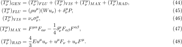
 = enthalpy,
  = Kronecker delta tensor,
  = pressure,
  = kinematic viscosity,
 = shear,
  = Faraday electromagnetic field tensor,
  = radiation energy density, and
 = radiation flux. In the remainder of this section we describe these components one by one, including
the most relevant details. Most models of accretion disks are given by steady-state solutions of the
conservation equations (43), with particular choices of the form of the stress-energy tensor
= radiation flux. In the remainder of this section we describe these components one by one, including
the most relevant details. Most models of accretion disks are given by steady-state solutions of the
conservation equations (43), with particular choices of the form of the stress-energy tensor  , and a
corresponding choice of the supplementary material equations. For example, thick accretion
disk models (Section 4) often assume
, and a
corresponding choice of the supplementary material equations. For example, thick accretion
disk models (Section 4) often assume  , thin disk models
(Section 5) assume
, thin disk models
(Section 5) assume 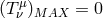 , and most current numerical models (Section 11) assume
 .
.
3.1 The fluid part
The one absolutely essential piece of the stress-energy tensor for describing accretion disks is the fluid part,
 . The fluid density, enthalpy, and pressure, as well as other fluid
characteristics, are linked by the first law of thermodynamics,
. The fluid density, enthalpy, and pressure, as well as other fluid
characteristics, are linked by the first law of thermodynamics,  , which we write in the
form,
, which we write in the
form,

 is the internal energy,
  is the temperature,
  is the entropy, and
  is the total
energy density, with
is the total
energy density, with  being the internal energy density, and
The equation of state is often assumed to be that of an ideal gas,
with
being the internal energy density, and
The equation of state is often assumed to be that of an ideal gas,
with 

 being the gas constant and
  the mean molecular weight.
Sometimes we may wish to consider a two temperature fluid, where the temperature  and molecular
weight
and molecular
weight  of the ions are different from those of the electrons (
 and
and  ). For such a case

3.1.1 Perfect fluid
In the case of a perfect fluid, the whole stress-energy tensor (44) is given by its fluid part (45),
and all other parts vanish, i.e., 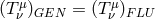 . In this particular case, one can use
 , and similarly derived
  , to prove that

 as the Bernoulli function and
  as the angular momentum.
Their ratio is obviously also a constant of motion,
identical in form with the specific angular momentum (7c), which is a constant of geodesic
motion.
as the angular momentum.
Their ratio is obviously also a constant of motion,
identical in form with the specific angular momentum (7c), which is a constant of geodesic
motion.

3.2 The stress part
In the stress part  , the shear tensor
  is a kinematic invariant (cf. Footnote 12). It is
defined as
is a kinematic invariant (cf. Footnote 12). It is
defined as
![[1 ] σμν ≡ --(∇ μuν + ∇ νuμ) − Θgμν (55 ) 2 ⊥](article326x.gif)
 denotes projection into the instantaneous 3-space perpendicular to
  in the sense
that
in the sense
that  . The other kinematic invariants are vorticity,
and expansion,
. The other kinematic invariants are vorticity,
and expansion,


In the standard hydrodynamical description (e.g. [168]), the viscous stress tensor,  , is proportional
to the shear tensor,
, is proportional
to the shear tensor,

 is then given by
In addition, the rates of viscous angular momentum and energy transport across a surface
is then given by
In addition, the rates of viscous angular momentum and energy transport across a surface 
 , with a unit
normal vector
, with a unit
normal vector  , are
, are

For the case of purely circular motion, where  , the kinematic invariants are

 . It is a general property that
  , and so for purely circular motion,
one has,
From Eqs. (60
, and so for purely circular motion,
one has,
From Eqs. (60 ) and (62) one deduces that for purely circular motion, the rates of energy and angular
momentum transport are related as
where
) and (62) one deduces that for purely circular motion, the rates of energy and angular
momentum transport are related as
where 
 is the angular velocity averaged on the surface
  . From this, one sees that as angular
momentum is transported outward, additional energy is carried inward by the fluid.
. From this, one sees that as angular
momentum is transported outward, additional energy is carried inward by the fluid.
3.2.1 The alpha viscosity prescription
As we mentioned in Section 1, the viscosity in astrophysical accretion disks can not come from ordinary molecular viscosity, as this is orders of magnitude too weak to explain observed phenomena. Instead, the source of stresses in the disk is likely turbulence driven by the magneto-rotational instability (MRI, described in Section 8.2). Even so, one can still parametrize the stresses within the disk as an effective viscosity and use the normal machinery of standard hydrodynamics without the complication of magnetohydrodynamics (MHD). This is sometimes desirable as analytic treatments of MHD can be very difficult to work with and full numerical treatments can be costly.
For these reasons, the Shakura–Sunyaev “alpha viscosity” prescription [279 ] still finds application today.
It is an ad hoc assumption based on dimensional arguments. Shakura and Sunyaev realized that if the
source of viscosity in accretion disks is turbulence, then the kinematic viscosity coefficient
] still finds application today.
It is an ad hoc assumption based on dimensional arguments. Shakura and Sunyaev realized that if the
source of viscosity in accretion disks is turbulence, then the kinematic viscosity coefficient  has the
form,
has the
form,

 is the correlation length of turbulence and
  is the mean turbulent speed. Assuming that the
velocity of turbulent elements cannot exceed the sound speed,
is the mean turbulent speed. Assuming that the
velocity of turbulent elements cannot exceed the sound speed,  , and that their typical size cannot
be greater than the disk thickness,
, and that their typical size cannot
be greater than the disk thickness,  , one gets
where
, one gets
where 
 is a dimensionless coefficient, assumed by Shakura and Sunyaev to be a
constant.
is a dimensionless coefficient, assumed by Shakura and Sunyaev to be a
constant.
For thin accretion disks (see Section 5) the viscous stress tensor reduces to an internal torque with the
following approximate form [see Eqs. (55) and (58)]

 and
and  , so Shakura and Sunyaev argued
that the torque must have the form
, so Shakura and Sunyaev argued
that the torque must have the form  . A critical question that was left unanswered was what
pressure
. A critical question that was left unanswered was what
pressure  one should consider:
  ,
,  , or
, or  ? This question has
now been answered using numerical simulations [128], so that we now know the appropriate
pressure to be
? This question has
now been answered using numerical simulations [128], so that we now know the appropriate
pressure to be  . Typical values of
  estimated from magnetohydrodynamic simulations are
close to 0.02 [122], while observations suggest a value closer to 0.1 (see [148] and references
therein).
estimated from magnetohydrodynamic simulations are
close to 0.02 [122], while observations suggest a value closer to 0.1 (see [148] and references
therein).
3.3 The Maxwell part
Magnetic fields may play many interesting roles in black hole accretion disks. Large scale magnetic fields
threading a disk may exert a torque, thereby extracting angular momentum [48]. Similarly, large scale
poloidal magnetic fields threading the inner disk, ergosphere, or black hole, have been shown to be able to
carry energy and angular momentum away from the system, and power jets [49]. Weak magnetic fields can
tap the differential rotation of the disk itself to amplify and trigger an instability that leads to turbulence,
angular momentum transport, and energy dissipation (exactly the processes that are needed for accretion to
happen) [26, 27].
In most black hole accretion disks, it is reasonable to assume ideal MHD, whereby the conductivity is infinite, and consequently the magnetic diffusivity is zero. Whenever this is true, magnetic field lines are effectively frozen into the fluid. A corollary to this is that parcels of fluid are restricted to moving along field lines, like “beads” on a wire. In ideal MHD, the Faraday tensor obeys the homogeneous Maxwell’s equation
where
 is the dual. If we define a magnetic field 4-vector
  , then using
  one can
show that
Using this, it is easy to show that the spatial components of (67
one can
show that
Using this, it is easy to show that the spatial components of (67 ) give the induction equation
while the time component gives the divergence-free constraint
where
) give the induction equation
while the time component gives the divergence-free constraint
where ![∂ (√ −-gBi) = − ∂ [√ −-g(Bivj − Bjvi )], (69 ) t j](article370x.gif)

 , and
, and  is the 4-metric determinant.
3.3.1 The magneto-rotational instability (MRI)
We mentioned in Section 3.2 that a hydrodynamic treatment of accretion requires an internal viscous stress
tensor of the form  . However, we also pointed out that ordinary molecular viscosity is too weak to
provide the necessary level of stress. Another possible source is turbulence. The mean stress from turbulence
always has the property that
. However, we also pointed out that ordinary molecular viscosity is too weak to
provide the necessary level of stress. Another possible source is turbulence. The mean stress from turbulence
always has the property that  , and so it can act as an effective viscosity. As we will explain in
Section 8.2, weak magnetic fields inside a disk are able to tap the shear energy of its differential
rotation to power turbulent fluctuations. This happens through a mechanism known as the
magneto-rotational (or “Balbus–Hawley”) instability [26, 118, 27]. Although the non-linear
behavior of the MRI and the turbulence it generates is quite complicated, its net effect on the
accretion disk can, in principle, be characterized as an effective viscosity, possibly making the
treatment much simpler. However, no such complete treatment has been developed at this
time.
, and so it can act as an effective viscosity. As we will explain in
Section 8.2, weak magnetic fields inside a disk are able to tap the shear energy of its differential
rotation to power turbulent fluctuations. This happens through a mechanism known as the
magneto-rotational (or “Balbus–Hawley”) instability [26, 118, 27]. Although the non-linear
behavior of the MRI and the turbulence it generates is quite complicated, its net effect on the
accretion disk can, in principle, be characterized as an effective viscosity, possibly making the
treatment much simpler. However, no such complete treatment has been developed at this
time.
3.4 The radiation part
Radiation is important in accretion disks as a way to carry excess energy away from the system. In geometrically thin, optically thick (Shakura–Sunyaev) accretion disks (Section 5.3), radiation is highly efficient and nearly all of the heat generated within the disk is radiated locally. Thus, the disk remains relatively cold. In other cases, such as ADAFs (Section 7), radiation is inefficient; such disks often remain geometrically thick and optically thin.
In the optically thin limit, the radiation emissivity  has the following components: bremsstrahlung
 , synchrotron
  , and their Comptonized parts
  and
and  . In the optically thick limit,
one often uses the diffusion approximation with the total optical depth
. In the optically thick limit,
one often uses the diffusion approximation with the total optical depth  coming from
the absorption and electron scattering optical depths. In the two limits, the emissivity is then
coming from
the absorption and electron scattering optical depths. In the two limits, the emissivity is then

 is the Stefan–Boltzmann constant. In the intermediate case one should solve the transfer
equation to get reliable results, as has been done in [288, 66]. Often, though, the solution of the grey
problem obtained by Hubeny [133] can serve reliably:
In sophisticated software packages like BHSPEC, color temperature corrections in the optically thick case (the
“hardening factor”) are often applied [66].
is the Stefan–Boltzmann constant. In the intermediate case one should solve the transfer
equation to get reliable results, as has been done in [288, 66]. Often, though, the solution of the grey
problem obtained by Hubeny [133] can serve reliably:
In sophisticated software packages like BHSPEC, color temperature corrections in the optically thick case (the
“hardening factor”) are often applied [66].
![4[ √ -- 4 ]−1 f = 4σTe-- 3τ-+ 3 + 4σT-e-(fbr + fsynch + fbr,C + fsynch,C )−1 . (72 ) H 2 H](article384x.gif)
In the remaining parts of this section we give explicit formulae for the bremsstrahlung and synchrotron
emissivities and their Compton enhancements. These sections are taken almost directly from the work of
Narayan and Yi [225]. Additional derivations and discussions of these equations in the black hole accretion
disk context may be found in [299, 295, 225, 87].
3.4.1 Bremsstrahlung
Thermal bremsstrahlung (or free-free emission) is caused by the inelastic scattering of relativistic thermal
electrons off (nonrelativistic) ions and other electrons. The emissivity (emission rate per unit volume) is
 . The ion-electron part is given by [225]
![{ ( ) 2 4 2𝜃e3-1∕2(1 + 1.781𝜃1e.34) 𝜃e < 1, fei = ne¯nσT cαfmec × 9𝜃eπ (73 ) 2π [ln(1.123𝜃e + 0.48) + 1.5] 𝜃e ≥ 1.](article386x.gif)
 is the electron number density,
  is the ion number density averaged over all species,
 is the Thomson cross section,
  is the fine structure constant,
 is the dimensionless electron temperature, and
  is the Boltzmann constant. The
electron-electron part is given by [225]
where
is the Boltzmann constant. The
electron-electron part is given by [225]
where ![{ 2 2 2 92π01∕2(44 − 3π2 )𝜃3∕e2(1 + 1.1𝜃e + 𝜃2e − 1.25𝜃5e∕2) 𝜃e < 1, fee = necremec αf × (74 ) 24𝜃e[ln (1.1232 𝜃e) + 1.28] 𝜃e ≥ 1.](article393x.gif)
 is the classical radius of the electron.
3.4.2 Synchrotron
Assuming the accretion environment is threaded by magnetic fields, the hot (relativistic) electrons can also
radiate via synchrotron emission. For a relativistic Maxwellian distribution of electrons, the formula is [225]
![[ 2 ] − 2π- d-- 3eB-𝜃exM-- fsynch = 3c2kTe dr 4πmec , (75 )](article395x.gif)
 is the electric charge,
  is the equipartition magnetic field strength, and
  is the solution
of the transcendental equation
where the radius
is the solution
of the transcendental equation
where the radius 
 must be in physical units and
  is the modified Bessel function of the second kind.
This expression is valid only for
is the modified Bessel function of the second kind.
This expression is valid only for  , but that is sufficient in most applications.
3.4.3 Comptonization
The hot, relativistic electrons can also Compton up-scatter the photons emitted via bremsstrahlung and
synchrotron radiation. The formulae for this are [225]
![{ [ ] } η1xc 3η1 3−(η3+1) − (3𝜃e)−(η3+1) fbr,C = fbr η1 − -3𝜃--− ----------η--+-1----------- (77 ) e 3 fsynch,C = fsynch[η1 − η2 (xc∕𝜃e)η3]. (78 )](article403x.gif)
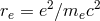
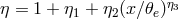 is the Compton energy enhancement factor, and
where
is the Compton energy enhancement factor, and
where 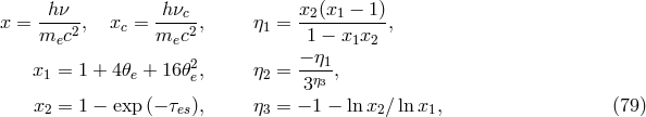
 is Planck’s constant and
  is the critical frequency, below which it is assumed that the
emission is completely self-absorbed and above which the emission is assumed to be optically
thin.
is the critical frequency, below which it is assumed that the
emission is completely self-absorbed and above which the emission is assumed to be optically
thin.
 |
 |
 |
Living Rev. Relativity, 16 (2013), 1, doi:10.12942/lrr-2013-1, URL (accessed <date>): http://www.livingreviews.org/lrr-2013-1.
 This work is licensed under a Creative Commons License.
© The author(s), except where otherwise noted.
This work is licensed under a Creative Commons License.
© The author(s), except where otherwise noted.