9 Oscillations
Even when analytic disk solutions are stable against finite perturbations, it is often the case that these perturbations will, nevertheless, excite oscillatory behavior. Oscillations are a common dynamical response in many fluid (and solid) bodies. Here we briefly explore the nature of oscillations in accretion disks. This topic is particularly relevant to understanding the physical mechanisms that may be behind quasi-periodic oscillations (or QPOs, which are discussed in Section 12.4).There are a number of local restoring forces available in accretion disks to drive oscillations. Local pressure gradients can drive oscillations via sound waves. Buoyancy forces can act through gravity waves. The Coriolis force can operate through inertial waves. Surface waves can also exist, with the restoring force given by the local effective gravity.
Of particular interest are families of low order modes that may exist in various accretion geometries. Such modes will tend to have the largest amplitudes and produce more easily observed changes than their higher-order counterparts. Here we briefly review a couple relatively simple examples for the purpose of illustration. More details can be found in the references given.
9.1 Dynamical oscillations of thick disks
A complete analysis of the spectrum of modes in thick disks has not yet been done. Some progress has been
made by considering the limiting case of a slender torus, where slender here means that the thickness of the
torus is small compared to its radial separation from the central mass (i.e., the torus has a small
cross-sectional area). In this limit, the complete set of modes have been determined for the case of constant
specific angular momentum in a Newtonian gravitational potential [43]. A more general analysis of slender
torus modes is given in [45 ].
].
Any finite, hydrodynamic flow orbiting a black hole, such as the Polish doughnuts described in
Section 4, is susceptible to axisymmetric, incompressible modes corresponding to global oscillations at the
radial ( ) and vertical (
 ) epicyclic frequencies. Other accessible modes are found by solving
the relativistic Papaloizou–Pringle equation [4]
) epicyclic frequencies. Other accessible modes are found by solving
the relativistic Papaloizou–Pringle equation [4]
![1 { [ ]} ( ) ----1∕2- ∂i (− g)1∕2gijfn∂jW − m2g ϕϕ − 2m ωgtϕ + ω2gtt fnW (− g) (ut)2(ω − m Ω )2 n−1 = − --------2-------f W , (108 ) cs0](article665x.gif)
 is defined by
![P P0 1 [ ℰ2 ] --= ---f(r,𝜃), f (r,𝜃 ) = 1 − --2- -0(𝒰eff − 𝒰eff,0) + Φ , (109 ) ρ ρ0 ncs0 2](article667x.gif)
 is the azimuthal wave number,
  is the polytropic index (assuming an equation of state of the form
 ),
),  is the sound speed at the pressure maximum
  , and
, and  is the determinant of the
metric. The necessary boundary condition comes from requiring that the Lagrangian pressure perturbation
vanish at the unperturbed surface (
is the determinant of the
metric. The necessary boundary condition comes from requiring that the Lagrangian pressure perturbation
vanish at the unperturbed surface ( ):
where
):
where 
 is the Lagrangian displacement vector. Eqs. (108
 ) and (110) describe a global eigenvalue
problem for the modes of Polish doughnuts, with three characteristic frequencies: the radial epicyclic
frequency
) and (110) describe a global eigenvalue
problem for the modes of Polish doughnuts, with three characteristic frequencies: the radial epicyclic
frequency  , the vertical epicyclic frequency
  , and the characteristic frequency of inertial modes
 .
.
In the slender-torus limit, one can write down analytic expressions for a few of the lowest order
modes [45] besides just the radial and vertical epicyclic ones. In terms of local coordinates measured from
the equilibrium point,

 , for some constant
  , yields two modes with eigenfrequencies [45]
where
, yields two modes with eigenfrequencies [45]
where ![2 1-{ 2 2 [ 2 2 2 2 2]1∕2} ¯σ0 = 2 ω r + ω 𝜃 ± (ω r + ω𝜃) + 4 κ0ω𝜃 , (112 )](article683x.gif)
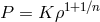
 . The positive square root gives a surface gravity mode that has the appearance of a
cross(
. The positive square root gives a surface gravity mode that has the appearance of a
cross( )-mode. The negative square root gives a purely incompressible inertial (c-) mode, whose poloidal
velocity field represents a circulation around the pressure maximum.
)-mode. The negative square root gives a purely incompressible inertial (c-) mode, whose poloidal
velocity field represents a circulation around the pressure maximum.
 ,
,  ) of the lowest order, non-trivial thick disk modes.
Image reproduced by permission from [45].
) of the lowest order, non-trivial thick disk modes.
Image reproduced by permission from [45]. An eigenfunction of the form  , with arbitrary constants
  , also has two
modes with eigenfrequencies [45]
, also has two
modes with eigenfrequencies [45]
![{ 2 1 2 2 2 ¯σ 0 = --- (2n + 1)(ωr + ω 𝜃) − (n + 1)κ 0 (113 ) 2n } [ 2 2 2 2 2 2 2 2]1∕2 ± ((2n + 1)(ω 𝜃 − ωr) + (n + 1)κ 0) + 4(ω r − κ 0)ω 𝜃 .](article691x.gif)
 , while in the
Keplerian limit, the mode frequency becomes that of a vertical acoustic wave. The lower sign corresponds to
a gravity wave, with a velocity field reminiscent of a plus(
, while in the
Keplerian limit, the mode frequency becomes that of a vertical acoustic wave. The lower sign corresponds to
a gravity wave, with a velocity field reminiscent of a plus( )-mode. The poloidal velocity fields of all
these lowest order modes are illustrated in Figure 13
)-mode. The poloidal velocity fields of all
these lowest order modes are illustrated in Figure 13 .
.
9.2 Diskoseismology: oscillations of thin disks
To analyze oscillations of thin disks, one can express the Eulerian perturbations of all physical quantities
through a single function  . Since the accretion disk is considered to be stationary and
axisymmetric, the angular and time dependence are factored out as
. Since the accretion disk is considered to be stationary and
axisymmetric, the angular and time dependence are factored out as 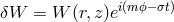 , where the
eigenfrequency
, where the
eigenfrequency 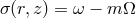 . Here it is useful to assume that the variation of the modes in the radial
direction is much stronger than in the vertical direction,
. Here it is useful to assume that the variation of the modes in the radial
direction is much stronger than in the vertical direction,  . The resulting two (separated)
differential equations for the functional amplitude
. The resulting two (separated)
differential equations for the functional amplitude 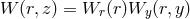 are given by [244, 311, 312]
![[ ] ( ) d2Wr 1 d ( 2 2) dWr (ut)2grr ( 2 2) Ψ ----2-− --2----2-- --- ω − ω r -----+ -------- ω − ωr 1 − -2- Wr = 0, (114 ) dr (ω − ωr) dr dr cs &tidle;ω 2 d2Wy-- dWy-- [ 2 2 2 ] (1 − y ) dy2 − 2gy dy + 2g &tidle;ω y + Ψ (1 − y ) Wy = 0. (115 )](article699x.gif)
 , varies rapidly with
  , while the vertical eigenfunction,
  , varies
slowly. Here
, varies
slowly. Here ![y = (z∕H )[γg∕(γg − 1)]1∕2](article703x.gif) is the re-scaled vertical coordinate,
is the re-scaled vertical coordinate,  is the adiabatic
index,
is the adiabatic
index, 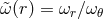 is the ratio of the epicyclic frequencies from Section 2.3,
  is the
eigenvalue of the (WKB) separation function, and
is the
eigenvalue of the (WKB) separation function, and 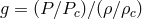 , where
  and
and  are the midplane values. The radial boundary conditions depend on the type of mode and its
capture zone (see below). Oscillations in thin accretion disks, then, are described in terms of
are the midplane values. The radial boundary conditions depend on the type of mode and its
capture zone (see below). Oscillations in thin accretion disks, then, are described in terms of
 , along with the angular, vertical, and radial mode numbers (number of nodes in the
corresponding eigenfunction)
, along with the angular, vertical, and radial mode numbers (number of nodes in the
corresponding eigenfunction)  ,
,  , and
, and  , respectively. Modes oscillate in the radial range where
outside the inner radius,
, respectively. Modes oscillate in the radial range where
outside the inner radius, 
 .
.
p-modes are inertial acoustic modes defined by  and are trapped where
  , which
occurs in two zones. The inner p-modes are trapped between the inner disk edge and the inner “Lindblad”
radius, i.e.,
, which
occurs in two zones. The inner p-modes are trapped between the inner disk edge and the inner “Lindblad”
radius, i.e.,  , where gas is accreted rapidly. The outer p-modes occur between the outer
Lindblad radius and the outer edge of the disk, i.e.,
, where gas is accreted rapidly. The outer p-modes occur between the outer
Lindblad radius and the outer edge of the disk, i.e.,  . The Lindblad radii,
  and
and
 , occur where
  . The outer p-modes are thought to be more consequential as they
produce stronger luminosity modulations [233]. In the corotating frame these modes appear at
frequencies slightly higher than the radial epicyclic frequency. Pressure is the main restoring force of
p-modes.
. The outer p-modes are thought to be more consequential as they
produce stronger luminosity modulations [233]. In the corotating frame these modes appear at
frequencies slightly higher than the radial epicyclic frequency. Pressure is the main restoring force of
p-modes.
g-modes are inertial gravity modes defined by  . They are trapped where
  in the
zone
in the
zone  given by the radial dependence of
  , i.e., g-modes are gravitationally captured in the
cavity of the radial epicyclic frequency and are thus the most robust among the thin-disk modes. Since this
is the region where the temperature of the disk peaks, g-modes are also expected to be most important
observationally [244]. In the corotating frame these modes appear at low frequencies. Gravity is their main
restoring force.
, i.e., g-modes are gravitationally captured in the
cavity of the radial epicyclic frequency and are thus the most robust among the thin-disk modes. Since this
is the region where the temperature of the disk peaks, g-modes are also expected to be most important
observationally [244]. In the corotating frame these modes appear at low frequencies. Gravity is their main
restoring force.
c-modes are corrugation modes defined by  . They are non-radial (
 ) and vertically
incompressible modes that appear near the inner disk edge and precess slowly around the rotational axis.
These modes are controlled by the radial dependence of the vertical epicyclic frequency. In the corotating
frame they appear at the highest frequencies.
) and vertically
incompressible modes that appear near the inner disk edge and precess slowly around the rotational axis.
These modes are controlled by the radial dependence of the vertical epicyclic frequency. In the corotating
frame they appear at the highest frequencies.
All modes have frequencies  . Upon the introduction of a small viscosity (
 ), most
of the modes grow on a dynamical timescale
), most
of the modes grow on a dynamical timescale  , such that the disk should become unstable. However,
evidence for these modes has so far mostly been lacking in MRI turbulent simulations (see Section 11.6).
This leaves their relevance in some doubt.
, such that the disk should become unstable. However,
evidence for these modes has so far mostly been lacking in MRI turbulent simulations (see Section 11.6).
This leaves their relevance in some doubt.
 |
 |
 |
Living Rev. Relativity, 16 (2013), 1, doi:10.12942/lrr-2013-1, URL (accessed <date>): http://www.livingreviews.org/lrr-2013-1.
 This work is licensed under a Creative Commons License.
© The author(s), except where otherwise noted.
This work is licensed under a Creative Commons License.
© The author(s), except where otherwise noted.