4 Thick Disks, Polish Doughnuts, & Magnetized Tori
In this section we discuss the simplest analytic model of a black hole accretion disk – the “Polish doughnut.” It is simplest in the sense that it only considers gravity (Section 2), plus a perfect fluid (Section 3.1.1), i.e., the absolute minimal description of accretion. We include magnetized tori in Section 4.2, which allows for , but otherwise
  throughout this section.
4.1 Polish doughnuts
Paczyński and his collaborators developed, in the late 1970s and early 1980s, a very general method of constructing perfect fluid equilibria of matter orbiting around a Kerr black hole [139, 236, 235, 234]. They assumed for the stress energy tensor and four velocity,
and derived from
 that,
In the case of a barytropic fluid
that,
In the case of a barytropic fluid 
 , the right-hand side of Eq. (81
 ) is the gradient of a scalar
function, and thus the left-hand side must also be the gradient of a scalar, which is possible if and only if
This statement is one of several useful integrability conditions, collectively called von Zeipel theorems, found
by a number of authors [51, 29, 1, 156
) is the gradient of a scalar
function, and thus the left-hand side must also be the gradient of a scalar, which is possible if and only if
This statement is one of several useful integrability conditions, collectively called von Zeipel theorems, found
by a number of authors [51, 29, 1, 156
 ].
].
In real flows, the function  is determined by dissipative processes that have timescales much
longer than the dynamical timescale, and are not yet fully understood. Paczyński realized that instead of
deriving
is determined by dissipative processes that have timescales much
longer than the dynamical timescale, and are not yet fully understood. Paczyński realized that instead of
deriving  from unsure assumptions about viscosity that involve a free function fixed
ad hoc (e.g., by assuming
from unsure assumptions about viscosity that involve a free function fixed
ad hoc (e.g., by assuming  const), one may instead assume the result, i.e., assume
 . Assuming
  is not self-consistent, but neither is assuming
  const.
In Boyer–Lindquist coordinates, the equation for the equipressure surfaces,  const, may
be written as
const, may
be written as  , with the function
  given by

 ,
,  , and
, and  from Section 2 (Eqs. 21 and 22),
one can integrate Eq. (83) to get the equipressure surfaces. A description of how to do this for both
Schwarzschild and Kerr black holes is given in [57]. Figure 4
from Section 2 (Eqs. 21 and 22),
one can integrate Eq. (83) to get the equipressure surfaces. A description of how to do this for both
Schwarzschild and Kerr black holes is given in [57]. Figure 4 illustrates the simplest (and important) case
of
illustrates the simplest (and important) case
of  .
.
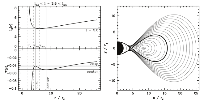
 , are circles on which the pressure gradient vanishes.
Thus, the (constant) angular momentum of matter equals the Keplerian angular momentum at these
two circles,
, are circles on which the pressure gradient vanishes.
Thus, the (constant) angular momentum of matter equals the Keplerian angular momentum at these
two circles,  , as shown in the upper left panel. In this figure
  refers
to the effective potential. Image reproduced by permission from [98], copyright by RAS.
refers
to the effective potential. Image reproduced by permission from [98], copyright by RAS. Another useful way to think about thick disks is from the relativistic analog of the Newtonian effective
potential  ,
,

 is the potential at the boundary of the thick disk. For constant angular momentum
  , the
form of the potential reduces to
, the
form of the potential reduces to  . Provided
  , the potential
  will have a
saddle point
will have a
saddle point  at
at  ,
,  . We can define the parameter
  as the
potential barrier (energy gap) at the inner edge of the disk. If
as the
potential barrier (energy gap) at the inner edge of the disk. If  , the disk lies entirely within its
Roche lobe, whereas if
, the disk lies entirely within its
Roche lobe, whereas if  , matter will spill into the black hole even without any loss of angular
momentum.
, matter will spill into the black hole even without any loss of angular
momentum.
Before leaving the topic of Polish doughnuts, we should point out that, starting with the work of
Hawley, Smarr, and Wilson [125], this simple, analytic solution has been the most commonly used starting
condition for numerical studies of black hole accretion.
4.2 Magnetized Tori
Komissarov [156] was able to extend the Polish doughnut solution by adding a purely azimuthal magnetic
field to create a magnetized torus. This is possible because a magnetic field of this form only enters the
equilibrium solution as an additional pressure-like term. For example, the extended form of Eq. (81) is

 and Eq. (84) becomes
where
and Eq. (84) becomes
where 
 . Komissarov [156] gives a procedure for solving the case of a barotropic magnetized
torus with constant angular momentum (
. Komissarov [156] gives a procedure for solving the case of a barotropic magnetized
torus with constant angular momentum ( const.).
 |
 |
 |
Living Rev. Relativity, 16 (2013), 1, doi:10.12942/lrr-2013-1, URL (accessed <date>): http://www.livingreviews.org/lrr-2013-1.
 This work is licensed under a Creative Commons License.
© The author(s), except where otherwise noted.
This work is licensed under a Creative Commons License.
© The author(s), except where otherwise noted.