List of Figures
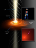 |
Figure 1:
An artist’s rendition of a generic black hole accretion disk and jet. Inset figures include a time sequence of radio images from the jet in microquasar, GRS 1915+105 [204] and an optical image of the jet in quasar, M87 (Credit: J.A. Biretta et al., Hubble Heritage Team (STScI /AURA), NASA). |
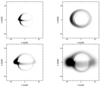 |
Figure 2:
Silhouettes of Sgr A* calculated for four optically thin accretion structures, characterized by very different physical conditions. The display is intentionally reversed in black-and-white and saturated in order to better show the less luminous parts. Although “dirty astrophysics” makes the most prominent differences, effects of the “pure strong gravity” are also seen in the form of “the light circle”, a tiny almost circular feature at the center. Its shape and size depends only on the black hole mass and spin. Image reproduced by permission from [297], copyright by ESO. |
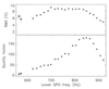 |
Figure 3:
Evidence for the existence of the ISCO from data recorded by the Rossi X-ray Timing Explorer satellite from neutron star binary source 4U 1636–536 [33]. The source shows quasi-periodic oscillations (QPOs) with frequencies in the range  . The sharp drop in the
quality factor (bottom panel) seen at . The sharp drop in the
quality factor (bottom panel) seen at  may be attributable to the ISCO [34]. may be attributable to the ISCO [34]. |
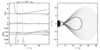 |
Figure 4:
In equilibrium, the equipressure surfaces should coincide with the surfaces shown by the solid lines in the right panel. Note the Roche lobe, self-crossing at the cusp. The cusp and the center, both located at the equatorial plane  , are circles on which the pressure gradient vanishes.
Thus, the (constant) angular momentum of matter equals the Keplerian angular momentum at these
two circles, , are circles on which the pressure gradient vanishes.
Thus, the (constant) angular momentum of matter equals the Keplerian angular momentum at these
two circles,  , as shown in the upper left panel. In this figure , as shown in the upper left panel. In this figure  refers
to the effective potential. Image reproduced by permission from [98], copyright by RAS. refers
to the effective potential. Image reproduced by permission from [98], copyright by RAS. |
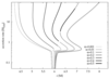 |
Figure 5:
Location of the sonic point as a function of the accretion rate for different values of  ,
for a non-rotating black hole, ,
for a non-rotating black hole,  , taking , taking  . The solid curves are for saddle
type solutions while the dotted curves present nodal type regimes. Image reproduced by permission
from [9], copyright by ESO. . The solid curves are for saddle
type solutions while the dotted curves present nodal type regimes. Image reproduced by permission
from [9], copyright by ESO. |
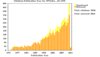 |
Figure 6:
The number of citations to the Shakura & Sunyaev paper [279] is still growing exponentially, implying that the field of black hole accretion disk theory still has not reached saturation. Image reproduced from the SAO/NASA Astrophysics Data System, URL (accessed 9 Jan 2013):  http://adsabs.harvard.edu/abs/1973A&A....24..337S. http://adsabs.harvard.edu/abs/1973A&A....24..337S. |
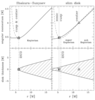 |
Figure 7:
The innermost part of the disk. In the Shakura–Sunyaev and Novikov–Thorne models, the locations of the maximum pressure (a.k.a. the center)  and the cusp and the cusp  , as well
as the sonic radius , as well
as the sonic radius  , are assumed to coincide with the ISCO. Furthermore, the angular
momentum is assumed to be strictly Keplerian outside the ISCO and constant inside it. In real
flows, , are assumed to coincide with the ISCO. Furthermore, the angular
momentum is assumed to be strictly Keplerian outside the ISCO and constant inside it. In real
flows,  , and angular momentum is super-Keplerian between , and angular momentum is super-Keplerian between  and
and  . Image reproduced by permission from [9], copyright by ESO. . Image reproduced by permission from [9], copyright by ESO. |
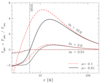 |
Figure 8:
The advection factor (ratio of advective to radiative cooling) profiles for  , ,
 and and  (here, (here,  ). Profiles for ). Profiles for  and and  are presented with
solid black and dashed red lines, respectively. The fraction are presented with
solid black and dashed red lines, respectively. The fraction  ) of heat generated by
viscosity is carried along with the flow. In regions with ) of heat generated by
viscosity is carried along with the flow. In regions with  the advected heat is released.
Image reproduced by permission from [269]. the advected heat is released.
Image reproduced by permission from [269]. |
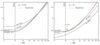 |
Figure 9:
Profiles of the disk angular momentum (  ) for ) for  (left) and (left) and  (right
panel) for different accretion rates (as a reminder, (right
panel) for different accretion rates (as a reminder,  ), showing the departures from
the Keplerian profile. These plots are for a non-rotating black hole. Image reproduced by permission
from [270], copyright by ESO. ), showing the departures from
the Keplerian profile. These plots are for a non-rotating black hole. Image reproduced by permission
from [270], copyright by ESO. |
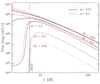 |
Figure 10:
Flux profiles for different mass accretion rates in the case of a non-rotating black hole and two values of  : 0.01 (black solid), 0.1 (red dashed lines). For each value of : 0.01 (black solid), 0.1 (red dashed lines). For each value of  there are five
lines corresponding to the following mass accretion rates: there are five
lines corresponding to the following mass accretion rates:  = 0.01, 0.1, 1.0, 2.0 and 10.0 (as a
reminder, = 0.01, 0.1, 1.0, 2.0 and 10.0 (as a
reminder,  ). The black hole mass is ). The black hole mass is  . Image reproduced by permission
from [270], copyright by ESO. . Image reproduced by permission
from [270], copyright by ESO. |
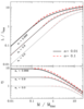 |
Figure 11:
Top panel: Luminosity vs accretion rate for three values of black hole spin (  , ,  , ,  ) and two values of ) and two values of  (black) and 0.1 (red line).
Bottom panel: efficiency of accretion (black) and 0.1 (red line).
Bottom panel: efficiency of accretion  (here (here  ). Image
reproduced by permission from [269]. ). Image
reproduced by permission from [269]. |
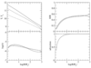 |
Figure 12:
Profiles of temperature, optical depth, ratio of scale height to radius, and advection factor (the ratio of advective cooling to turbulent heating) of a hot, one-  ADAF (solid lines). The
parameters are ADAF (solid lines). The
parameters are  , ,  , ,  , and , and  .
The outer boundary conditions are .
The outer boundary conditions are  , ,  , and , and  . Two- . Two- solutions with the same parameters and
  (dashed lines) and 0.01 (dot-dashed lines) are also
shown for comparison, where (dashed lines) and 0.01 (dot-dashed lines) are also
shown for comparison, where  is the fraction of the turbulent viscous energy that directly heats
the electrons. Image reproduced by permission from [321], copyright by AAS. is the fraction of the turbulent viscous energy that directly heats
the electrons. Image reproduced by permission from [321], copyright by AAS. |
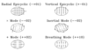 |
Figure 13:
Poloidal velocity fields (  , ,  ) of the lowest order, non-trivial thick disk modes.
Image reproduced by permission from [45]. ) of the lowest order, non-trivial thick disk modes.
Image reproduced by permission from [45]. |
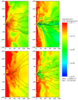 |
Figure 14:
Pseudo-color plots of  with contours of with contours of  from four different general
relativistic MHD simulations. The simulations all begin with the same initial conditions, but have
different energy conservation and cooling treatments: The upper-left panel conserves internal energy
and ignores cooling; the upper-right panel conserves internal energy and includes cooling; the
lower-left panel conserves total energy and ignores cooling; the lower-right panel conserves total
energy and includes cooling. The very different end states illustrate the importance of properly
capturing thermodynamic processes. Image reproduced by permission from [101], copyright by AAS. from four different general
relativistic MHD simulations. The simulations all begin with the same initial conditions, but have
different energy conservation and cooling treatments: The upper-left panel conserves internal energy
and ignores cooling; the upper-right panel conserves internal energy and includes cooling; the
lower-left panel conserves total energy and ignores cooling; the lower-right panel conserves total
energy and includes cooling. The very different end states illustrate the importance of properly
capturing thermodynamic processes. Image reproduced by permission from [101], copyright by AAS. |
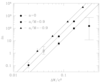 |
Figure 15:
Time-average mass accretion rate  as a function of the energy gap as a function of the energy gap  for models with
  (circles), (circles),  (squares), and (squares), and  (triangles). The bars
show the variability of (triangles). The bars
show the variability of  . The lines represent the predicted dependencies . The lines represent the predicted dependencies  ,
where ,
where  is the adiabatic index. Image reproduced by permission from [137], copyright by
RAS. is the adiabatic index. Image reproduced by permission from [137], copyright by
RAS. |
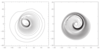 |
Figure 16:
Equatorial slice through hydrodynamic tori at saturation of the Papaloizou–Pringle instability showing formation of significant non-axisymmetric (  ) overdensity clumps. The
density contours are linearly spaced between ) overdensity clumps. The
density contours are linearly spaced between  and 0.0. This figure represents models A3p (left)
and B3r (right) of [69]. Image reproduced by permission, copyright by AAS. and 0.0. This figure represents models A3p (left)
and B3r (right) of [69]. Image reproduced by permission, copyright by AAS. |
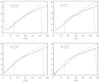 |
Figure 17:
Specific angular momentum  as a function of radius at as a function of radius at  (thin line) and at (thin line) and at
 orbits (thick line). The individual plots are labeled by model. In each case the Keplerian
distribution for a test particle, orbits (thick line). The individual plots are labeled by model. In each case the Keplerian
distribution for a test particle,  , is shown as a dashed line. Image reproduced by permission
from [72], copyright by AAS. , is shown as a dashed line. Image reproduced by permission
from [72], copyright by AAS. |
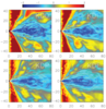 |
Figure 18:
Color contours of the ratio of azimuthally averaged magnetic to gas pressure,  .
The scale is logarithmic and is the same for all panels; the color maps saturate in the axial funnel. The
body of the accretion disk is identified with overlaid density contours at .
The scale is logarithmic and is the same for all panels; the color maps saturate in the axial funnel. The
body of the accretion disk is identified with overlaid density contours at  , ,  , ,  ,
and ,
and  of of  . The individual plots are labeled by model. In all cases, the magnetic
pressure is low ( . The individual plots are labeled by model. In all cases, the magnetic
pressure is low ( ) in the disk, comparable to gas pressure ( ) in the disk, comparable to gas pressure ( ) in the
corona above and below the disk, and high ( ) in the
corona above and below the disk, and high ( ) in the funnel region. Image reproduced
by permission from [72], copyright by AAS. ) in the funnel region. Image reproduced
by permission from [72], copyright by AAS. |
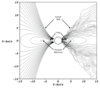 |
Figure 19:
On the left, equidensity contours calculated from an analytic Polish doughnut. On the right, equidensity contours from a numerical MHD simulation (model 90h from [99]). Note, though, that the contours on the left are linearly spaced, while those on the right are logarithmically spaced. Thus, the gradients represented on the left are shallower than those on the right. Image reproduced by permission from [253], copyright by ESO. |
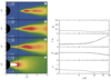 |
Figure 20:
Left: Time-averaged rest mass density in the  – –  plane for four GRMHD simulations
with plane for four GRMHD simulations
with  and various disk thicknesses. The dashed vertical line marks the ISCO. The disk opening
angle, and various disk thicknesses. The dashed vertical line marks the ISCO. The disk opening
angle,  , and effective Shakura–Sunyaev viscosity, , and effective Shakura–Sunyaev viscosity,  , are reported in each panel. The
top three panels have , are reported in each panel. The
top three panels have  and the inner edge of the disk is located outside the ISCO. The
bottom panel has and the inner edge of the disk is located outside the ISCO. The
bottom panel has  and the density increases monotonically down to the event horizon.
Figure from [241]. Right: Various fluxes as functions of radius for a numerical Novikov–Thorne disk
simulation. Top: Mass accretion rate. Second panel: Accreted specific angular momentum. Solid line
is simulation data; dashed line gives Novikov–Thorne solution; dotted line is ISCO value. Note that
the specific angular momentum does not drop significantly inside the ISCO, unlike for thick disks,
such as in Figure 17. Third panel: The “nominal” efficiency, which is the total loss of specific energy
from the fluid. Bottom panel: Specific magnetic flux. The near constancy of this quantity inside the
ISCO is an indication that magnetic stresses are not significant in this region. Image reproduced by
permission from [240]. and the density increases monotonically down to the event horizon.
Figure from [241]. Right: Various fluxes as functions of radius for a numerical Novikov–Thorne disk
simulation. Top: Mass accretion rate. Second panel: Accreted specific angular momentum. Solid line
is simulation data; dashed line gives Novikov–Thorne solution; dotted line is ISCO value. Note that
the specific angular momentum does not drop significantly inside the ISCO, unlike for thick disks,
such as in Figure 17. Third panel: The “nominal” efficiency, which is the total loss of specific energy
from the fluid. Bottom panel: Specific magnetic flux. The near constancy of this quantity inside the
ISCO is an indication that magnetic stresses are not significant in this region. Image reproduced by
permission from [240]. |
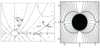 |
Figure 21:
On the left is a schematic diagram of the Blandford–Znajek mechanism [49] for an assumed parabolic field distribution. On the right is the result of a numerical simulation from [158] showing a very similar structure. Images reproduced by permission; copyright RAS. |
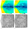 |
Figure 22:
Top: Distributions of density in the meridional plane at different simulation times, showing a magnetically arrested state (left) and a non-arrested state (right). Bottom: Snapshot of magnetic field lines at the same simulation times. Image reproduced by permission from [135], copyright by AAS. |
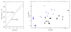 |
Figure 23:
Left: Luminosity as a function of accretion rate for neutron star and black hole sources, illustrating that a wider range of luminosities are expected for black holes. Image reproduced by permission from [215], copyright by AAS. Right: Recent data showing that neutron star sources (open symbols) are systematically more luminous than black hole sources (filled symbols) in analogous spectral states. Image reproduced by permission from [171], copyright by Elsevier. |
Marek A. Abramowicz and P. Chris Fragile, "Foundations of Black Hole Accretion Disk Theory",
Living Rev. Relativity, 16 (2013), 1, doi:10.12942/lrr-2013-1, URL (accessed <date>): http://www.livingreviews.org/lrr-2013-1. This work is licensed under a Creative Commons License.
© The author(s), except where otherwise noted.
This work is licensed under a Creative Commons License.
© The author(s), except where otherwise noted.
Living Rev. Relativity, 16 (2013), 1, doi:10.12942/lrr-2013-1, URL (accessed <date>): http://www.livingreviews.org/lrr-2013-1.
This work is licensed under a Creative Commons License.
© The author(s), except where otherwise noted.