2 Three Destinations in Kerr’s Strong Gravity
In this section, we briefly describe the three destinations within Kerr’s strong gravity that are most relevant to black hole accretion disk theory:- Event Horizon: That radius inside of which escape from the black hole is not possible;
- Ergosphere: That radius inside of which negative energy states are possible (giving rise to the potentiality of tapping the energy of the black hole).
- Innermost Stable Circular Orbit (ISCO): That radius inside of which free circular orbital motion is not possible;
Our principal question is: Could accretion disk theory unambiguously prove the existence of the event horizon, ergosphere, and ISCO using currently available or future observations?
In realistic astrophysical situations involving astrophysical black holes (in particular quasars and
microquasars), the black hole itself is uncharged, and the gravity of accretion disk is practically negligible.
This means that the spacetime metric  is given by the Kerr metric, determined by two
parameters: total mass
is given by the Kerr metric, determined by two
parameters: total mass  and total angular momentum
  . It is convenient to rescale them by
such that both  and
and  are measured in units of length.
In the standard spherical Boyer–Lindquist coordinates the Kerr metric takes the form [31 ],
],
 and
and  .
.
The Kerr metric depends neither on time  , nor on the azimuthal angle
  around the symmetry
axis. These two symmetries can be expressed in a coordinate independent way by the two commuting
Killing vectors
around the symmetry
axis. These two symmetries can be expressed in a coordinate independent way by the two commuting
Killing vectors  and
and  ,
,

Here  denotes the covariant derivative,

 denotes the standard partial derivative. Formulae for the Kerr metric (3
 ) and all its
non-zero Christoffell symbols
) and all its
non-zero Christoffell symbols  (5), are available from [305].
In Boyer–Lindquist coordinates the  and
and  components of the Kerr metric can be expressed as
scalar products of the Killing vectors,
components of the Kerr metric can be expressed as
scalar products of the Killing vectors,


The Carter constant  is connected to the Killing tensor
  , which exists in the Kerr metric.
Killing tensors obey,
, which exists in the Kerr metric.
Killing tensors obey,
![1- 6 [∇ κK μν + ∇ μK νκ + ∇ νK κμ + ∇ κK νμ + ∇νK μκ + ∇ μK κν] = 0. (8 )](article115x.gif)
 is a unit vector, and
  is given implicitly by the condition,
Note that we have given the Kerr–Schild metric in its Cartesian form to prevent confusion with the
spherical-polar Boyer–Lindquist coordinates. In keeping with this, unless specifically stated
otherwise, the indices
is given implicitly by the condition,
Note that we have given the Kerr–Schild metric in its Cartesian form to prevent confusion with the
spherical-polar Boyer–Lindquist coordinates. In keeping with this, unless specifically stated
otherwise, the indices 
 will always refer to the Boyer–Lindquist coordinates in this
review.
will always refer to the Boyer–Lindquist coordinates in this
review.
2.1 The event horizon
The mathematically precise, general, definition of the event horizon involves topological considerations [207]. Here, we give a definition which is less general, but in the specific case of the Kerr geometry is fully equivalent.
The Boyer–Lindquist coordinates split the Kerr spacetime into a “time” coordinate  and a
three-dimensional “space,” defined as
and a
three-dimensional “space,” defined as  hypersurfaces. This split may be done in a coordinate
independent way, based on the Killing vectors which exist in the Kerr spacetime. Indeed, the family of
non-geodesic observers
hypersurfaces. This split may be done in a coordinate
independent way, based on the Killing vectors which exist in the Kerr spacetime. Indeed, the family of
non-geodesic observers  with trajectories orthogonal to a family of 3-D spaces
  is defined
as,
is defined
as,
They are called zero-angular-momentum-observers (ZAMO), because for them, the angular momentum
defined by (7b) is zero,  . The ZAMO observers provide the standard of rest in the 3-D
space: objects motionless with respect to the ZAMO frame of reference occupy fixed positions in
space.
. The ZAMO observers provide the standard of rest in the 3-D
space: objects motionless with respect to the ZAMO frame of reference occupy fixed positions in
space.
We can also define a gravitational potential in the ZAMO frame:
The primary reason to call![[ ] 1 ξμξμ 1 tt potential: Φ ≡ − --ln --ν---2----ν-----μ---- = − --ln |g |. (12 ) 2 (η ξν) − (η η ν)(ξ ξμ ) 2](article127x.gif)
 the gravitational potential is that, in Newton’s theory, the observer who
stays still in space experiences an acceleration due to “gravity”
the gravitational potential is that, in Newton’s theory, the observer who
stays still in space experiences an acceleration due to “gravity”  , which equals the gradient of the
gravitational potential. In the Kerr spacetime it is,
From (11a) one sees that at the surface
, which equals the gradient of the
gravitational potential. In the Kerr spacetime it is,
From (11a) one sees that at the surface 
 , the vector
  is null,
  . Therefore,
the ZAMO observers who provide the standard of rest, move on that surface with the speed
of light. In order to stand still in this location, one must move radially out with the speed of
light.11
As it is clear from (3),
. Therefore,
the ZAMO observers who provide the standard of rest, move on that surface with the speed
of light. In order to stand still in this location, one must move radially out with the speed of
light.11
As it is clear from (3),  is equivalent to
  . The last equation has a double solution,
Note, that for
. The last equation has a double solution,
Note, that for 
 the ZAMO “observers” are spacelike: standing still at a given radial location implies
moving along a spacelike trajectory – i.e., faster than light. All trajectories that move radially out are also
spacelike. Thus, the outer root
the ZAMO “observers” are spacelike: standing still at a given radial location implies
moving along a spacelike trajectory – i.e., faster than light. All trajectories that move radially out are also
spacelike. Thus, the outer root  of Eq. (14) defines the Kerr black hole event horizon: a null
surface that surrounds a region from which nothing may escape. Outside the outer horizon (i.e., for
of Eq. (14) defines the Kerr black hole event horizon: a null
surface that surrounds a region from which nothing may escape. Outside the outer horizon (i.e., for
 ) the normalization of
  is non-singular, and therefore the gravitational potential (12) is a
non-singular, well-defined quantity.
is non-singular, and therefore the gravitational potential (12) is a
non-singular, well-defined quantity.
2.1.1 Detecting the event horizon
One may think of two general classes of astrophysical observations that could provide evidence for a black hole horizon. Arguments in the first class are indirect; they are based on estimating a dimensionless “compactness parameter”
Arguments in the second class are more direct. They are based (in principle) on showing that some amount of radiation emitted by the source is lost inside the horizon.
Evidence based on estimating the compactness parameter: A source for which observations indicate
 may be suspected of having an event horizon. Values
  have indeed been found in several
astronomical sources. In order to know
have indeed been found in several
astronomical sources. In order to know  , one must know mass and size of the source. The mass
measurement is usually a direct one, because it may be based on an application of Kepler’s
laws. In a few cases the mass measurement is remarkably accurate. For example, in the case of
Sgr A*, the supermassive black hole in the center of our Galaxy, the mass is measured to be
, one must know mass and size of the source. The mass
measurement is usually a direct one, because it may be based on an application of Kepler’s
laws. In a few cases the mass measurement is remarkably accurate. For example, in the case of
Sgr A*, the supermassive black hole in the center of our Galaxy, the mass is measured to be
 [111].
Until recently, estimates of size were always indirect, and generally not accurate. They are usually based
on time variability or spectral considerations. For the former, the measurement rests on the logic that if the
shortest observed variability time-scale is  , then the size of the source cannot be larger than
 . For the latter, the argument goes like this: If the total radiative power
  and
the radiative flux
and
the radiative flux  can be independently measured for a black-body source, then its size
can be estimated from
can be independently measured for a black-body source, then its size
can be estimated from  . Keep in mind that one must know the distance to the
source in order to measure
. Keep in mind that one must know the distance to the
source in order to measure  . The flux can be estimated from
  , where
  is the
temperature corresponding to the peak in the observed intensity versus frequency electromagnetic
spectrum.
is the
temperature corresponding to the peak in the observed intensity versus frequency electromagnetic
spectrum.
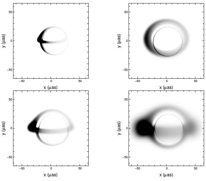
It is hoped that in the near future, the next generation of high-tech radio telescopes will be able to
measure directly the size of “the light circle”, which is uniquely related to the horizon size (see Figure 2 ).
For Sgr A*, at a distance of
).
For Sgr A*, at a distance of  [111], the event horizon corresponds to an angular size of
 in the sky, making it an ideal target for near-future microarcsecond very long base
interferometric techniques [77, 83]. Here the plan is to measure the black hole “shadow” or
“silhouette.”
in the sky, making it an ideal target for near-future microarcsecond very long base
interferometric techniques [77, 83]. Here the plan is to measure the black hole “shadow” or
“silhouette.”
Evidence based on the “no escape” argument: For accretion onto an object with a physical surface (such
as a star), 100% of the gravitational binding energy released by accretion must be radiated away. This does
not apply for a black hole since the event horizon allows for the energy to be advected into the hole
without being radiated. This may allow for a black hole with an event horizon to be distinguished
from another, similar-mass object with a surface, such as a neutron star. This argument was
first developed by Narayan and collaborators [215, 216, 214]; we describe it in more detail in
Section 12.2.
2.2 The ergosphere
In Newtonian gravity, angular momentum  and angular velocity
  are related by the formula
 , and therefore there is no ambiguity in defining a non-rotating frame as
  . However, in
the Kerr geometry
. However, in
the Kerr geometry  , where
  is the angular velocity of the frame dragging
induced by the Lense–Thirring effect. Therefore,
is the angular velocity of the frame dragging
induced by the Lense–Thirring effect. Therefore,  does not imply
  . This leads to two
different standards of “rotational rest”: the Zero Angular Velocity Observer (ZAVO) and the Zero Angular
Momentum Observer (ZAMO),
. This leads to two
different standards of “rotational rest”: the Zero Angular Velocity Observer (ZAVO) and the Zero Angular
Momentum Observer (ZAMO),

 .
.
The ZAMO frame defines a local standard of rest with respect to the local compass of inertia:
a gyroscope stationary in the ZAMO frame does not precess. Considering its kinematic
invariants,12
one sees that the ZAMO frame is non-inertial ( ), non-rigid (
 ,
,  ), and
surface-forming (
), and
surface-forming ( ). The ZAMO vectors
  and
and  are time-like everywhere outside the
horizon, i.e., outside the surface
are time-like everywhere outside the
horizon, i.e., outside the surface  . This means that the energy of a particle or photon with a
four-momentum
. This means that the energy of a particle or photon with a
four-momentum  measured by the ZAMO is positive,
  .
.
The ZAVO frame defines a global standard of rest with respect to distant stars: a telescope that points
to a fixed star does not rotate in the ZAVO frame. Considering its kinematic invariants one sees that the
ZAVO frame is non-inertial ( ), rigid (
 ,
,  ), and not surface-forming
(
), and not surface-forming
( ). At infinity, i.e., for
  , it is
  , and therefore
  .
For this reason,
.
For this reason,  is called the stationary observer at infinity. The ZAVO vectors
  and
and
 are timelike outside the region surrounded by the surface
  , called the ergosphere.
Inside the ergosphere
, called the ergosphere.
Inside the ergosphere  and
and  are spacelike. This means that inside the ergosphere, the
conserved energy of a particle (i.e., the energy measured “at infinity”), as defined by (7a), may be
negative.
are spacelike. This means that inside the ergosphere, the
conserved energy of a particle (i.e., the energy measured “at infinity”), as defined by (7a), may be
negative.
Penrose [242] considered a process in which, inside the ergosphere, a particle with energy  decays into two particles with energies
  and
and  . The particle with positive
energy escapes to infinity, and the particle with the negative energy gets absorbed by the black hole. Then,
because
. The particle with positive
energy escapes to infinity, and the particle with the negative energy gets absorbed by the black hole. Then,
because  , one gets a net gain of positive energy at infinity. The source of
energy in this Penrose process is the rotational energy of the black hole. Indeed, the angular momentum
absorbed by the black hole,
, one gets a net gain of positive energy at infinity. The source of
energy in this Penrose process is the rotational energy of the black hole. Indeed, the angular momentum
absorbed by the black hole,  is necessarily negative (in the sense that
  , which
follows from
, which
follows from

and thus
A more complete presentation of the Penrose process is made in [310]. At this time it appears the most likely realization of the Penrose process would be the Blandford–Znajek mechanism [49 ] for launching jets
from quasars and microquasars. Observations suggest [255, 252], and simulations confirm [303, 304], that
through this mechanism it is possible to extract more energy from the system than is being delivered
by accretion. We discuss jets and the Blandford-Znajek mechanism more in Sections 10 and
11.7.
] for launching jets
from quasars and microquasars. Observations suggest [255, 252], and simulations confirm [303, 304], that
through this mechanism it is possible to extract more energy from the system than is being delivered
by accretion. We discuss jets and the Blandford-Znajek mechanism more in Sections 10 and
11.7.
2.3 ISCO: the orbit of marginal stability
Particles (with velocity normalization  ) and photons (with velocity normalization
  )
move freely on “geodesic” trajectories
)
move freely on “geodesic” trajectories  , with velocities
  , characterized by
vanishing accelerations
, characterized by
vanishing accelerations

 , such as those defined in Eq. (7), is conserved along a geodesic trajectory (19) in
the sense that
, such as those defined in Eq. (7), is conserved along a geodesic trajectory (19) in
the sense that  .
.
Circular geodesic motion in the equatorial plane ( ) is of fundamental importance in black
hole accretion disk theory. The four velocity corresponding to circular motion is defined by,
) is of fundamental importance in black
hole accretion disk theory. The four velocity corresponding to circular motion is defined by,

 is the angular velocity measured by the stationary observer (ZAVO, see
Section 2.2), and the redshift factor,
is the angular velocity measured by the stationary observer (ZAVO, see
Section 2.2), and the redshift factor,  , follows from
  ,
Other connections between these quantities that are particularly useful in our later calculations also follow
from
,
Other connections between these quantities that are particularly useful in our later calculations also follow
from 
 :
It is convenient to define the effective potential,
because in terms of
:
It is convenient to define the effective potential,
because in terms of 

 and the rescaled energy
  , slightly non-circular motion, i.e., with
 , is characterized by the equation,
which has the same form and the same physical meaning as the corresponding Newtonian equation.
Therefore, exactly as in Newtonian theory, unperturbed circular Keplerian orbits are given by
the condition of an extremum (minimum or maximum) of the effective potential
, is characterized by the equation,
which has the same form and the same physical meaning as the corresponding Newtonian equation.
Therefore, exactly as in Newtonian theory, unperturbed circular Keplerian orbits are given by
the condition of an extremum (minimum or maximum) of the effective potential 
 ,
This quadratic equation for
,
This quadratic equation for 
 has two roots
  , corresponding to “corotating”
and “counterrotating” Keplerian orbits. Their explicit algebraic form is given in Eq. (35) in
Section 2.5.
, corresponding to “corotating”
and “counterrotating” Keplerian orbits. Their explicit algebraic form is given in Eq. (35) in
Section 2.5.
As in Newtonian theory, slightly non-circular orbits (with  being either
  or
or  ) are fully
determined by the simple harmonic oscillator equations,
) are fully
determined by the simple harmonic oscillator equations,

 and vertical
  epicyclic frequencies are second derivatives of the effective potential,
where
epicyclic frequencies are second derivatives of the effective potential,
where 
 . The epicyclic frequencies (27) are measured by the comoving observer. To get the
frequencies
. The epicyclic frequencies (27) are measured by the comoving observer. To get the
frequencies  measured by the stationary “observer at infinity” (Section 2.2), one must rescale by the
redshift factor
measured by the stationary “observer at infinity” (Section 2.2), one must rescale by the
redshift factor  . Obviously, when
  , the epicyclic radial oscillations described by
Eq. (26) are unstable – from Eq. (27) we see that they correspond to maxima of the effective potential.
This happens for all circular orbits with radii less than
, the epicyclic radial oscillations described by
Eq. (26) are unstable – from Eq. (27) we see that they correspond to maxima of the effective potential.
This happens for all circular orbits with radii less than  , and this limiting radius is called ISCO,
the innermost stable circular orbit.
, and this limiting radius is called ISCO,
the innermost stable circular orbit.
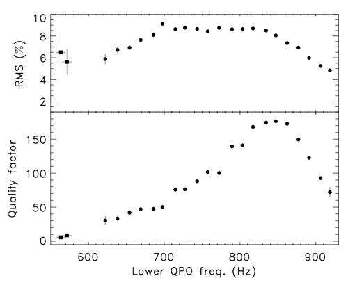 ]. The source shows quasi-periodic
oscillations (QPOs) with frequencies in the range
]. The source shows quasi-periodic
oscillations (QPOs) with frequencies in the range  . The sharp drop in the
quality factor (bottom panel) seen at
. The sharp drop in the
quality factor (bottom panel) seen at  may be attributable to the ISCO [34].
 Free circular orbits with  are stable, while those with
  are not. Accordingly, accretion
flows of almost free matter (i.e., with stresses insignificant in comparison with gravity or centrifugal
effects), resemble almost circular motion for
are not. Accordingly, accretion
flows of almost free matter (i.e., with stresses insignificant in comparison with gravity or centrifugal
effects), resemble almost circular motion for  , and almost radial free-fall for
  .
For thin disks, this transition in the character of the flow is expected to produce an effective
inner truncation radius in the disk (see Section 5.3). The exceptional stability of the inner
radius of the X-ray binary LMC X-3 [293], provides considerable evidence for such a connection
and, hence, for the existence of the ISCO. The transition of the flow at the ISCO may also
show up in the observed variability pattern, if variability is modulated by the orbital motion.
In this case, one may expect that the there will be no variability observed with frequencies
.
For thin disks, this transition in the character of the flow is expected to produce an effective
inner truncation radius in the disk (see Section 5.3). The exceptional stability of the inner
radius of the X-ray binary LMC X-3 [293], provides considerable evidence for such a connection
and, hence, for the existence of the ISCO. The transition of the flow at the ISCO may also
show up in the observed variability pattern, if variability is modulated by the orbital motion.
In this case, one may expect that the there will be no variability observed with frequencies
 , i.e., higher than the Keplerian orbital frequency at ISCO, or that the quality factor for
variability,
, i.e., higher than the Keplerian orbital frequency at ISCO, or that the quality factor for
variability,  will significantly drop at
  . Several variants of this idea have been
discussed [33, 34], and some observational evidence to support them has been presented (see
Figure 3).
. Several variants of this idea have been
discussed [33, 34], and some observational evidence to support them has been presented (see
Figure 3).
2.4 The Paczyński–Wiita potential
For a non-rotating black hole ( ), the Kerr metric reduces to the Schwarzschild solution,
![( ) ( )− 1 2 2M-- 2 2M-- 2 2[ 2 2 2] ds = − 1 − r dt + 1 − r dr + r d𝜃 + sin 𝜃d ϕ . (28 )](article259x.gif) ] proposed a practical and accurate Newtonian model for a Schwarzschild black
hole, based on the gravitational potential,
The Paczyński–Wiita potential became a very handy tool for studying black hole astrophysics. It has been
used in many papers on the subject and still has applicability today. The Schwarzschild and
the Paczyński–Wiita expressions for the Keplerian angular momentum and locations of the
marginally stable and marginally bound orbits (Section 2.3) are identical. Similar, though less
commonly adopted, pseudo-Newtonian potentials have also been found for Kerr (rotating) black
holes [23, 276, 213].
] proposed a practical and accurate Newtonian model for a Schwarzschild black
hole, based on the gravitational potential,
The Paczyński–Wiita potential became a very handy tool for studying black hole astrophysics. It has been
used in many papers on the subject and still has applicability today. The Schwarzschild and
the Paczyński–Wiita expressions for the Keplerian angular momentum and locations of the
marginally stable and marginally bound orbits (Section 2.3) are identical. Similar, though less
commonly adopted, pseudo-Newtonian potentials have also been found for Kerr (rotating) black
holes [23, 276, 213].

2.5 Summary: characteristic radii and frequencies
We end this section with a few formulae for the Kerr geometry that we will use elsewhere in this review.
Keplerian circular orbits exist in the region  , with
  being the circular photon orbit. Bound
orbits exist in the region
being the circular photon orbit. Bound
orbits exist in the region  , with
  being the marginally bound orbit, and stable orbits exist for
 , with
  being the marginally stable orbit (also called the ISCO – Section 2.3). The location
of these radii, as well as the location of the horizon
being the marginally stable orbit (also called the ISCO – Section 2.3). The location
of these radii, as well as the location of the horizon  and ergosphere
  , are given by the following
formulae [31]:
, are given by the following
formulae [31]:
![{ [ ]} 2 −1 photon rph = 2rG 1 + cos 3-cos (a∗) , (30 ) ( √ ------) bound rmb = 2rG 1 − a∗-+ 1 − a∗ , (31 ) { 2 } stable r = r 3 + Z − [(3 − Z )(3 + Z + 2Z )]1∕2 , (32 ) ms G ( 2 ) 1 1 2 ∘ -----2 horizon rH = rG 1 + 1 − a∗ , (33 ) ( ∘ -----2---2--) ergosphere r0 = rG 1 + 1 − a∗cos 𝜃 , (34 )](article269x.gif)
![2 1∕3 1∕3 1∕3 Z1 = 1 + (1 − a∗) [(1 + a∗) + (1 − a∗) ]](article270x.gif) ,
,  ,
,  , and
, and
 is the gravitational radius.
The Keplerian angular momentum  and angular velocity
  , and the angular velocity of frame
dragging
, and the angular velocity of frame
dragging  are given by,
 ),
Comparing the Keplerian and epicyclic frequencies and the characteristic radii between the Schwarzschild
metric and the Paczyński–Wiita potential (Section 2.4), we find for the Schwarzschild metric,
and for the Paczyński–Wiita potential,
),
Comparing the Keplerian and epicyclic frequencies and the characteristic radii between the Schwarzschild
metric and the Paczyński–Wiita potential (Section 2.4), we find for the Schwarzschild metric,
and for the Paczyński–Wiita potential,

 |
 |
 |
Living Rev. Relativity, 16 (2013), 1, doi:10.12942/lrr-2013-1, URL (accessed <date>): http://www.livingreviews.org/lrr-2013-1.
 This work is licensed under a Creative Commons License.
© The author(s), except where otherwise noted.
This work is licensed under a Creative Commons License.
© The author(s), except where otherwise noted.