5 Thin Disks
Most analytic accretion disk models assume a stationary and axially symmetric state of the matter being accreted into the black hole. In such models, all physical quantities depend only on the two spatial coordinates: the “radial” distance from the center , and the “vertical” distance from the equatorial
symmetry plane
, and the “vertical” distance from the equatorial
symmetry plane  . In addition, the most often studied models assume that the disk is not vertically thick.
In “thin” disks
. In addition, the most often studied models assume that the disk is not vertically thick.
In “thin” disks  everywhere inside the matter distribution, and in “slim” disks (Section 6)
 .
.
In thin and slim disk models, one often uses a vertically integrated form for many physical
quantities. For example, instead of density  one uses the surface density defined as,
 gives the location of the surface of the accretion disk.
5.1 Equations in the Kerr geometry
The general relativistic equations describing the physics of thin disks have been derived independently by
several authors [169, 7 , 13, 106, 40]. Here we present them in the form used in [268]:
- Mass conservation (continuity):
where
 is the gas radial velocity measured by an observer at fixed
  who co-rotates with the
fluid, and
who co-rotates with the
fluid, and  has the same meaning as in Section 2.
- Radial momentum conservation:
where
 ,
,  is the angular velocity with respect to the
stationary observer,
is the angular velocity with respect to the
stationary observer,  is the angular velocity with respect to the inertial observer,
 are the angular frequencies of the co-rotating and counter-rotating
Keplerian orbits, and
are the angular frequencies of the co-rotating and counter-rotating
Keplerian orbits, and  is the radius of gyration.
- Angular momentum conservation:
where
 is the specific angular momentum,
  is the Lorentz factor,
  can be
considered to be the vertically integrated pressure,
can be
considered to be the vertically integrated pressure,  is the standard alpha viscosity (Section 3.2.1),
and
is the standard alpha viscosity (Section 3.2.1),
and  is the specific angular momentum at the horizon, which can not be known a priori. As we
explain in the next section, it provides an eigenvalue linked to the unique eigensolution of the set of
thin disk differential equations, once they are properly constrained by boundary and regularity
conditions.
is the specific angular momentum at the horizon, which can not be known a priori. As we
explain in the next section, it provides an eigenvalue linked to the unique eigensolution of the set of
thin disk differential equations, once they are properly constrained by boundary and regularity
conditions.
- Vertical equilibrium:
with
 being the conserved energy associated with the time symmetry.
- Energy conservation:
where
 is the temperature in the equatorial plane,
  is the mean (frequency-independent)
opacity,
is the mean (frequency-independent)
opacity,

 ,
,  ,
,  , and
, and  is the
ratio of specific heats of the gas.
is the
ratio of specific heats of the gas.


5.2 The eigenvalue problem
Through a series of algebraic manipulations one can reduce the thin disk equations to a set of two ordinary
differential equations for two dependent variables, e.g., the Mach number  and the
angular momentum
and the
angular momentum  . Their structure reveals an important point here,
 and
and  must vanish at
the same radius as the denominator
must vanish at
the same radius as the denominator  . The denominator vanishes at the “sonic” radius
  where the Mach number is equal to unity, and the equation
  determines its
location.
determines its
location.
The extra regularity conditions at the sonic point  are satisfied only for one particular
value of the angular momentum at the horizon
are satisfied only for one particular
value of the angular momentum at the horizon  , which is the eigenvalue of the problem that should be
found. For a given
, which is the eigenvalue of the problem that should be
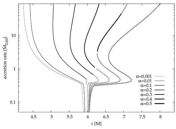
found. For a given  the location of the sonic point depends on the mass accretion rate. For low mass
accretion rates one expects the transonic transition to occur close to the ISCO. Figure 5
the location of the sonic point depends on the mass accretion rate. For low mass
accretion rates one expects the transonic transition to occur close to the ISCO. Figure 5 shows that
this is indeed the case for accretion rates smaller than about
shows that
this is indeed the case for accretion rates smaller than about  , independent of
  ,
where we use the authors’ definition of
,
where we use the authors’ definition of  . At
. At  a qualitative
change occurs, resembling a “phase transition” from the Shakura–Sunyaev behavior to a very
different slim-disk behavior. For higher accretion rates the location of the sonic point significantly
departs from the ISCO. For low values of
a qualitative
change occurs, resembling a “phase transition” from the Shakura–Sunyaev behavior to a very
different slim-disk behavior. For higher accretion rates the location of the sonic point significantly
departs from the ISCO. For low values of  , the sonic point moves closer to the horizon,
down to
, the sonic point moves closer to the horizon,
down to  for
for  . For
. For  the sonic point moves outward with increasing
accretion rate, reaching values as high as
the sonic point moves outward with increasing
accretion rate, reaching values as high as  for
for  and
and  . This effect
was first noticed for small accretion rates by Muchotrzeb [212] and later investigated for a
wide range of accretion rates by Abramowicz [10], who explained it in terms of the disk-Bondi
dichotomy.
. This effect
was first noticed for small accretion rates by Muchotrzeb [212] and later investigated for a
wide range of accretion rates by Abramowicz [10], who explained it in terms of the disk-Bondi
dichotomy.
 ,
for a non-rotating black hole,
,
for a non-rotating black hole,  , taking
  . The solid curves are for saddle
type solutions while the dotted curves present nodal type regimes. Image reproduced by permission
from [9], copyright by ESO.
. The solid curves are for saddle
type solutions while the dotted curves present nodal type regimes. Image reproduced by permission
from [9], copyright by ESO. The topology of the sonic point is important, because physically acceptable solutions must be of the
saddle or nodal type; the spiral type is forbidden. The topology may be classified by the eigenvalues
 of the Jacobi matrix,
 , only two eigenvalues
  are non-zero, and the quadratic characteristic equation
that determines them takes the form,
The nodal-type solution is given by
are non-zero, and the quadratic characteristic equation
that determines them takes the form,
The nodal-type solution is given by ![2 [ 2 2 ] 2λ − 2λtr(𝒥 ) − tr(𝒥 ) − tr (𝒥 ) = 0. (97 )](article517x.gif)
 and the saddle type by
  , as marked in Figure 5
with the dotted and the solid lines, respectively. For the lowest values of
, as marked in Figure 5
with the dotted and the solid lines, respectively. For the lowest values of  only the saddle-type solutions
exist. For moderate values of
only the saddle-type solutions
exist. For moderate values of  (
( ) the topological type of the sonic point changes at least
once with increasing accretion rate. For the highest
) the topological type of the sonic point changes at least
once with increasing accretion rate. For the highest  solutions, only nodal-type critical points
exist.
solutions, only nodal-type critical points
exist.
5.3 Solutions: Shakura–Sunyaev & Novikov–Thorne
Shakura and Sunyaev [279] noticed that a few physically reasonable extra assumptions reduce the system of
thin disk equations (88 ) – (93) to a set of algebraic equations. Indeed, the continuity and vertical
equilibrium equations, (88) and (92), are already algebraic. The radial momentum equation (90) becomes a
trivial identity
) – (93) to a set of algebraic equations. Indeed, the continuity and vertical
equilibrium equations, (88) and (92), are already algebraic. The radial momentum equation (90) becomes a
trivial identity  with the extra assumptions that the radial pressure and velocity gradients vanish,
and the rotation is Keplerian,
with the extra assumptions that the radial pressure and velocity gradients vanish,
and the rotation is Keplerian,  . The algebraic angular momentum equation (91) only requires
that we specify
. The algebraic angular momentum equation (91) only requires
that we specify  . The Shakura–Sunyaev model makes the assumption that
  . This is
equivalent to assuming that the torque vanishes at the ISCO. This is a point of great interest that has been
challenged repeatedly [164, 104, 25]. Direct testing of this hypothesis by numerical simulations is discussed
in Section 11.4.
. This is
equivalent to assuming that the torque vanishes at the ISCO. This is a point of great interest that has been
challenged repeatedly [164, 104, 25]. Direct testing of this hypothesis by numerical simulations is discussed
in Section 11.4.
The right-hand side of the energy equation (93) represents advective cooling. This is assumed to vanish
in the Shakura–Sunyaev model, though we will see that it plays a critical role in slim disks (Section 6) and
ADAFs (Section 7). Because the Shakura–Sunyaev model assumes the rotation is Keplerian,
 , meaning
  is a known function of
  , the first term on the left-hand side of
Eq. (93), which represents viscous heating, is algebraic. The second term, which represents the
radiative cooling (in the diffusive approximation) is also algebraic in the Shakura–Sunyaev
model.
, the first term on the left-hand side of
Eq. (93), which represents viscous heating, is algebraic. The second term, which represents the
radiative cooling (in the diffusive approximation) is also algebraic in the Shakura–Sunyaev
model.
In addition to being algebraic, these thin-disk equations are also linear in three distinct radial ranges:
outer, middle, and inner. Therefore, as Shakura and Sunyaev realized, the model may be given in terms of
explicit algebraic (polynomial) formulae. This was an achievement of remarkable consequences – still today
the understanding of accretion disk theory is in its major part based on the Shakura–Sunyaev
analytic model. The Shakura–Sunyaev paper [279] is one of the most cited in astrophysics
today (see Figure 6), illustrating how fundamentally important accretion disk theory is in the
field.
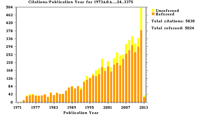
 http://adsabs.harvard.edu/abs/1973A&A....24..337S.
 The general relativistic version of the Shakura–Sunyaev disk model was worked out by Novikov and
Thorne [229], with important extensions and corrections provided in subsequent papers [237, 265, 241].
Here we reproduce the solution, although with a more general scaling:  and
and  .
.
Outer region:  ,
,  (free-free opacity)
r∗ ℬ 𝒞 𝒬, Σ = [4 × 10⁵ g cm −2](α−4∕5m2 ∕10m˙70∕∗10)r∗−3∕4𝒜1 ∕10ℬ −4∕5𝒞1∕2𝒟− 17∕20ℰ− 1∕20𝒬7 ∕10, 2 −1∕10 18∕20 3∕20 9∕8 19∕20 −11∕10 1∕2 −23∕40 −19∕40 3∕20 H = [4 × 10 cm ](α m m˙ )r∗ 𝒜 ℬ 𝒞 𝒟 ℰ 𝒬 , ρ0 = [4 × 10² g cm −3](α−7∕10m −7∕10m˙11 ∕20)r−∗ 15∕8𝒜 −17∕20ℬ3 ∕10𝒟 −11∕40ℰ 17∕40𝒬11∕20, T = [2 × 10⁸ K ](α−1∕5m −1∕5 ˙m3∕10)r−3∕4𝒜− 1∕10ℬ −1∕5𝒟 −3∕20ℰ1∕20𝒬3∕10, ∗ β ∕(1 − β) = [3](α −1∕10m −1∕10 ˙m −7∕20)r3∗∕8𝒜 −11∕20ℬ9∕10𝒟7 ∕40ℰ11∕40𝒬− 7∕20, τ ∕τ = [2 × 10 −3](m˙− 1∕2)r3∕4𝒜− 1∕2ℬ2 ∕5𝒟1 ∕4ℰ1∕4𝒬− 1∕2, (98 ) ff es ∗](article536x.gif)
 .
.
Middle region:  ,
,  (electron-scattering opacity)
r−3ℬ −1𝒞− 1∕2𝒬, ∗ Σ = [9 × 10⁴ g cm −2](α−4∕5m1 ∕5m˙3 ∕5)r−∗3∕5ℬ−4∕5𝒞1∕2𝒟 −4∕5𝒬3 ∕5, H = [1 × 103 cm ](α−1∕10m9∕10m˙1 ∕5)r21∕20𝒜 ℬ −6∕5𝒞1∕2𝒟 − 3∕5ℰ −1∕2𝒬1 ∕5, 1 −3 −7∕10 −7∕10 ∗2∕5 −33∕20 −1 3∕5 −1∕5 1∕2 2∕5 ρ0 = [4 × 10 g cm ](α m m˙ )r∗ 𝒜 ℬ 𝒟 ℰ 𝒬 , T = [7 × 10⁸ K ](α −1∕5m −1∕5m ˙2 ∕5)r−9∕10ℬ −2∕5𝒟 −1∕5𝒬2 ∕5, −3 −1∕10 −1∕10 −4∕5∗21∕20 − 1 9∕5 2∕5 1∕2 −4∕5 β ∕(1 − β) = [7 × 10 ](α m ˙m )r∗ 𝒜 ℬ 𝒟 ℰ 𝒬 , τff∕τes = [2 × 10 −6](m˙−1)r3∗∕2𝒜 −1ℬ2𝒟1 ∕2ℰ1∕2𝒬− 1, (99 )](article540x.gif)
Inner region:  ,
, 
r∗ ℬ 𝒞 𝒬, Σ = [5 g cm− 2](α− 1 ˙m −1)r3∗∕2𝒜 −2ℬ3 𝒞1∕2ℰ𝒬 −1, 5 2 −3 1∕2 −1 − 1 H = [1 × 10 cm](m˙)𝒜 ℬ 𝒞 𝒟 ℰ 𝒬, ρ0 = [2 × 10⁻⁵ g cm −3](α −1m −1m˙−2)r3∗∕2𝒜− 4ℬ6𝒟 ℰ2𝒬 −2, 7 − 1∕4 −1∕4 −3∕8 − 1∕2 1∕2 1∕4 T = [5 × 10 K](α m )r∗ 𝒜 ℬ ℰ , β∕(1 − β) = [4 × 10⁻⁶](α−1∕4m −1∕4 ˙m −2)r21∗∕8𝒜 −5∕2ℬ9∕2𝒟 ℰ5∕4𝒬− 2, (τ τ )1∕2 = [1 × 10⁻⁴](α−17∕16m − 1∕16m˙−2)r93∕32𝒜 −25∕8ℬ41∕8𝒞1∕2𝒟1 ∕2ℰ25∕16𝒬 −2. (100 ) ff es ∗](article543x.gif)
 that appear in Eqs. (98), (99), (100), are defined in terms of
  and
and  as [237]:
![[ 3 ( y ) 3(y1 − a∗)2 ( y − y1) ] 𝒬 = 𝒬0 y − y0 − --a∗ln -- − --------------------ln ------- [ 2 y0 (y1(y1 − y)2)(y1 − y3) y0 − y1 ( ) ] ----3(y2 −-a∗)2----- -y-−-y2 ----3-(y3-−-a∗)2----- y-−-y3- − 𝒬0 y (y − y )(y − y ) ln y − y − y (y − y )(y − y ) ln y − y 2 2 1 2 3 0 2 3 3 1 3 2 0 3](article548x.gif)
 , and
, and  ,
,  , and
, and  are the three roots of
  ; that is
![−1 y1 = 2cos[(cos a ∗ − π )∕3], y2 = 2cos[(cos−1a ∗ + π )∕3 ], −1 y3 = − 2cos[(cos a∗)∕3].](article554x.gif) , the opacities were assumed to be
, the opacities were assumed to be  and
and  , where
  is the density in
  and
and  is the
temperature in Kelvin.
is the
temperature in Kelvin.
The Shakura–Sunyaev and Novikov–Thorne solutions are only local solutions; this is because they
do not take into account the full eigenvalue problem described in Section 5.2. Instead, they
make an assumption that the viscous torque goes to zero at the ISCO, which makes the model
singular there. For very low accretion rates, this singularity of the model does not influence the
electromagnetic spectrum [298], nor several other important astrophysical predictions of the
model. However, in those astrophysical applications in which the inner boundary condition is
important (e.g., global modes of disk oscillations), the Novikov–Thorne model is inadequate.
Figure 7 illustrates a few ways in which the model fails to capture the true physics near the
ISCO.
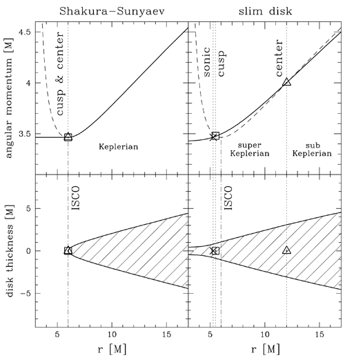
 and the cusp
  , as well
as the sonic radius
, as well
as the sonic radius  , are assumed to coincide with the ISCO. Furthermore, the angular
momentum is assumed to be strictly Keplerian outside the ISCO and constant inside it. In real
flows,
, are assumed to coincide with the ISCO. Furthermore, the angular
momentum is assumed to be strictly Keplerian outside the ISCO and constant inside it. In real
flows,  , and angular momentum is super-Keplerian between
  and
and  . Image reproduced by permission from [9], copyright by ESO.
 |
 |
 |
Living Rev. Relativity, 16 (2013), 1, doi:10.12942/lrr-2013-1, URL (accessed <date>): http://www.livingreviews.org/lrr-2013-1.
 This work is licensed under a Creative Commons License.
© The author(s), except where otherwise noted.
This work is licensed under a Creative Commons License.
© The author(s), except where otherwise noted.