2 Alternative Theories of Gravity
In this section, we discuss the many possible alternative theories that have been studied so far in the context of gravitational-wave tests. We begin with a description of the theoretically desirable properties that such theories must have. We then proceed with a review of the theories so far explored as far as gravitational waves are concerned. We will leave out the description of many theories in this chapter, especially those which currently lack a gravitational-wave analysis. We will conclude with a brief description of unexplored theories as possible avenues for future research.
2.1 Desirable theoretical properties
The space of possible theories is infinite, and thus, one is tempted to reduce it by considering a subspace that satisfies a certain number of properties. Although the number and details of such properties depend on the theorist’s taste, there is at least one fundamental property that all scientists would agree on:
- Precision Tests. The theory must produce predictions that pass all solar system, binary pulsar, cosmological and experimental tests that have been carried out so far.
This requirement can be further divided into the following:
-
- General Relativity Limit. There must exist some limit, continuous or discontinuous, such as the weak-field one, in which the predictions of the theory are consistent with those of GR within experimental precision.
- Existence of Known Solutions [426*]. The theory must admit solutions that correspond to observed phenomena, including but not limited to (nearly) flat spacetime, (nearly) Newtonian stars, and cosmological solutions.
- Stability of Solutions [426*]. The special solutions described in property (1.b) must be stable to small perturbations on timescales smaller than the age of the universe. For example, perturbations to (nearly) Newtonian stars, such as impact by asteroids, should not render such solutions unstable.
Of course, these properties are not all necessarily independent, as the existence of a weak-field limit usually also implies the existence of known solutions. On the other hand, the mere existence of solutions does not necessarily imply that these are stable.
In addition to these fundamental requirements, one might also wish to require that any new modified gravity theory possesses certain theoretical properties. These properties will vary depending on the theorist, but the two most common ones are listed below:
- Well-motivated from Fundamental Physics. There must be some fundamental theory or principle from which the modified theory (effective or not) derives. This fundamental theory would solve some fundamental problem in physics, such as late-time acceleration or the incompatibility between quantum mechanics and GR.
- Well-posed Initial Value Formulation [426]. A wide class of freely specifiable initial data must exist, such that there is a uniquely determined solution to the modified field equations that depends continuously on this data.
The second property goes without saying at some level, as one expects modified-gravity–theory constructions to be motivated from some (perhaps yet incomplete) quantum-gravitational description of nature. As for the third property, the continuity requirement is necessary because otherwise the theory would lose predictive power, given that initial conditions can only be measured to a finite accuracy. Moreover, small changes in the initial data should not lead to solutions outside the causal future of the data; that is, causality must be preserved. Section 2.2 expands on this well-posedness property further.
One might be concerned that Property (2) automatically implies that any predicted deviation to
astrophysical observables will be too small to be detectable. This argument usually goes as follows. Any
quantum gravitational correction to the action will “naturally” introduce at least one new scale, and this,
by dimensional analysis, must be the Planck scale. Since this scale is usually assumed to be larger than
1 TeV in natural units (or  in geometric units), gravitational-wave observations will never be able
to observe quantum-gravitational modifications (see, e.g., [155*] for a similar argument). Although this
might be true, in our view such arguments can be extremely dangerous, since they induce a certain
theoretical bias in the search for new phenomena. For example, let us consider the supernova
observations of the late-time expansion of the universe that led to the discovery of the cosmological
constant. The above argument certainly fails for the cosmological constant, which on dimensional
arguments is over 100 orders of magnitude too small. If the supernova teams had respected this
argument, they would not have searched for a cosmological constant in their data. Today, we try
to explain our way out of the failure of such dimensional arguments by claiming that there
must be some exquisite cancellation that renders the cosmological constant small; but this, of
course, came only after the constant had been measured. One is not trying to argue here that
cancellations of this type are common and that quantum gravitational modifications are necessarily
expected in gravitational-wave observations. Rather, we are arguing that one should remain
agnostic about what is expected and what is not, and allow oneself to be surprised without
suppressing the potential for new discoveries that will accompany the new era of gravitational-wave
astrophysics.
in geometric units), gravitational-wave observations will never be able
to observe quantum-gravitational modifications (see, e.g., [155*] for a similar argument). Although this
might be true, in our view such arguments can be extremely dangerous, since they induce a certain
theoretical bias in the search for new phenomena. For example, let us consider the supernova
observations of the late-time expansion of the universe that led to the discovery of the cosmological
constant. The above argument certainly fails for the cosmological constant, which on dimensional
arguments is over 100 orders of magnitude too small. If the supernova teams had respected this
argument, they would not have searched for a cosmological constant in their data. Today, we try
to explain our way out of the failure of such dimensional arguments by claiming that there
must be some exquisite cancellation that renders the cosmological constant small; but this, of
course, came only after the constant had been measured. One is not trying to argue here that
cancellations of this type are common and that quantum gravitational modifications are necessarily
expected in gravitational-wave observations. Rather, we are arguing that one should remain
agnostic about what is expected and what is not, and allow oneself to be surprised without
suppressing the potential for new discoveries that will accompany the new era of gravitational-wave
astrophysics.
One last property that we wish to consider for the purposes of this review is:
- Strong Field Inconsistency. The theory must lead to observable deviations from GR in the strong-field regime.
Many modified gravity models have been proposed that pose infrared or cosmological modifications to GR, aimed at explaining certain astrophysical or cosmological observables, like the late expansion of the universe. Such modified models usually reduce to GR in the strong-field regime, for example via a Vainshtein-like mechanism [413*, 140*, 45*] in a static spherically-symmetric context. Extending this mechanism to highly-dynamical strong-field scenarios has not been fully worked out yet [137*, 138*]. Gravitational-wave tests of GR, however, are concerned with modified theories that predict deviations in the strong-field, precisely where cosmological modified models do not. Clearly, Property (4) is not necessary for a theory to be a valid description of nature. This is because a theory might be identical to GR in the weak and strong fields, yet different at the Planck scale, where it would be unified with quantum mechanics. However, Property (4) is a desirable feature if one is to test this theory with gravitational wave observations.
2.2 Well-posedness and effective theories
Property (3) not only requires the existence of an initial value formulation, but also that it be well posed,
which is not necessarily guaranteed. For example, the Cauchy–Kowalewski theorem states that a system of
 partial differential equations for
  unknown functions
  of the form
  ,
with
,
with  analytic functions has an initial value formulation (see, e.g., [425*]). However, this theorem does
not guarantee continuity or the causal conditions described above. For this, one has to rely on more
general energy arguments, for example constructing a suitable energy measure that obeys the
dominant energy condition and using it to show well-posedness (see, e.g., [225, 425*]). One can
show that second-order, hyperbolic partial differential equations, i.e., equations of the form
analytic functions has an initial value formulation (see, e.g., [425*]). However, this theorem does
not guarantee continuity or the causal conditions described above. For this, one has to rely on more
general energy arguments, for example constructing a suitable energy measure that obeys the
dominant energy condition and using it to show well-posedness (see, e.g., [225, 425*]). One can
show that second-order, hyperbolic partial differential equations, i.e., equations of the form

 is an arbitrary vector field and
  are smooth functions, have a well-posed initial value
formulation. Moreover, the Leray theorem proves that any quasilinear, diagonal, second-order hyperbolic
system also has a well-posed initial value formulation [425*].
are smooth functions, have a well-posed initial value
formulation. Moreover, the Leray theorem proves that any quasilinear, diagonal, second-order hyperbolic
system also has a well-posed initial value formulation [425*].
Proving the well-posedness of an initial-value formulation for systems of higher-than-second-order, partial differential equations is much more difficult. In fact, to our knowledge, no general theorems exist of the type described above that apply to third, fourth or higher-order, partial, non-linear and coupled differential equations. Usually, one resorts to the Ostrogradski theorem [337*] to rule out (or at the very least cast serious doubt on) theories that lead to such higher-order field equations. Ostrogradski’s theorem states that Lagrangians that contain terms with higher-than-first-time derivatives possess a linear instability in the Hamiltonian (see, e.g., [443*] for a nice review).2 As an example, consider the Lagrangian density
whose equations of motion, obviously contain higher derivatives. The exact solution to this differential equation is where


 are constants and
 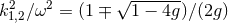 . The on-shell Hamiltonian is then

However, the Ostrogradski theorem [337] can be evaded if the Lagrangian in Eq. (6*) describes an
effective theory, i.e., a theory that is a truncation of a more general or complete theory. Let us reconsider
the particular example above, assuming now that the coupling constant  is an effective theory parameter
and Eq. (6*) is only valid to linear order in
is an effective theory parameter
and Eq. (6*) is only valid to linear order in  . One approach is to search for perturbative
solutions of the form
. One approach is to search for perturbative
solutions of the form  , which leads to the system of differential equations

 . Solving this set of
  differential equations and resumming, one finds

 contains only the positive (well-behaved) energy solution of Eq. (8*), i.e., perturbation
theory acts to retain only the well-behaved, stable solution of the full theory in the
contains only the positive (well-behaved) energy solution of Eq. (8*), i.e., perturbation
theory acts to retain only the well-behaved, stable solution of the full theory in the  limit. One
can also think of the perturbative theory as the full theory with additional constraints, i.e.,
the removal of unstable modes, which is why such an analysis is sometimes called perturbative
constraints [117, 118, 466*].
limit. One
can also think of the perturbative theory as the full theory with additional constraints, i.e.,
the removal of unstable modes, which is why such an analysis is sometimes called perturbative
constraints [117, 118, 466*].
Another way to approach effective field theories that lead to equations of motion with higher-order
derivatives is to apply the method of order reduction. In this method, one substitutes the low-order
derivatives of the field equations into the high-order derivative part, thus rendering the resulting new theory
usually well posed. One can think of this as a series resummation, where one changes the non-linear
behavior of a function by adding uncontrolled, higher-order terms. Let us provide an explicit example by
reconsidering the theory in Eq. (6*). To lowest order in  , the equation of motion is that of a simple
harmonic oscillator,
, the equation of motion is that of a simple
harmonic oscillator,


 . The solution to this
order-reduced differential equation is
. The solution to this
order-reduced differential equation is  once more, but with
  linearized in
  . Therefore, the
solutions obtained with a perturbative decomposition and with the order-reduced equation of motion are
the same to linear order in
. Therefore, the
solutions obtained with a perturbative decomposition and with the order-reduced equation of motion are
the same to linear order in  . Of course, since an effective field theory is only defined to a certain order in
its perturbative parameter, both treatments are equally valid, with the unstable mode effectively removed in
both cases.
. Of course, since an effective field theory is only defined to a certain order in
its perturbative parameter, both treatments are equally valid, with the unstable mode effectively removed in
both cases.
However, such a perturbative analysis can say nothing about the well-posedness of the full theory from
which the effective theory derives, or of the effective theory if treated as an exact one (i.e.,
not as a perturbative expansion). In fact, a well-posed full theory may have both stable and
unstable solutions. The arguments presented above only discuss the stability of solutions in an
effective theory, and thus, they are self-consistent only within their perturbative scheme. A full
theory may have non-perturbative instabilities, but these can only be studied once one has
a full (non-truncated in  ) theory, from which Eq. (6*) derives as a truncated expansion.
Lacking a full quantum theory of nature, quantum gravitational models are usually studied in a
truncated low-energy expansion, where the leading-order piece is GR and higher-order pieces
are multiplied by a small coupling constant. One can perturbatively explore the well-behaved
sector of the truncated theory about solutions to the leading-order theory. However, such an
analysis is incapable of answering questions about well-posedness or non-linear stability of the full
theory.
) theory, from which Eq. (6*) derives as a truncated expansion.
Lacking a full quantum theory of nature, quantum gravitational models are usually studied in a
truncated low-energy expansion, where the leading-order piece is GR and higher-order pieces
are multiplied by a small coupling constant. One can perturbatively explore the well-behaved
sector of the truncated theory about solutions to the leading-order theory. However, such an
analysis is incapable of answering questions about well-posedness or non-linear stability of the full
theory.
2.3 Explored theories
In this subsection we briefly describe the theories that have so far been studied in some depth as far as gravitational waves are concerned. In particular, we focus only on those theories that have been sufficiently studied so that predictions of the expected gravitational waveforms (the observables of gravitational-wave detectors) have been obtained for at least a typical source, such as the quasi-circular inspiral of a compact binary.
2.3.1 Scalar-tensor theories
Scalar-tensor theories in the Einstein frame [82, 129*, 166, 165, 181, 197] are defined by the action (where
we will restore Newton’s gravitational constant  in this section)
![∫ (E) 1 4 √--- μν 2 S ST = ------ d x − g [R − 2g (∂ μφ)(∂νφ ) − V(φ )] + Smat[ψmat,A (φ)gμν], (14 ) 16πG](article78x.gif)
 is a scalar field,
  is a coupling function,
  is a potential function,
  represents
matter degrees of freedom and
represents
matter degrees of freedom and  is Newton’s constant in the Einstein frame. For more details on this
theory, we refer the interested reader to the reviews [438*, 435*]. Of course, one can consider more
complicated scalar-tensor theories, for example by including multiple scalar fields, but we will ignore such
generalizations here.
is Newton’s constant in the Einstein frame. For more details on this
theory, we refer the interested reader to the reviews [438*, 435*]. Of course, one can consider more
complicated scalar-tensor theories, for example by including multiple scalar fields, but we will ignore such
generalizations here.
The Einstein frame is not the frame where the metric governs clocks and rods, and thus, it is convenient
to recast the theory in the Jordan frame through the conformal transformation 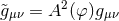 :
:
![1 ∫ ∘ ---[ ω (ϕ) ] S(SJT)= ------ d4x − &tidle;g ϕ &tidle;R − -----&tidle;gμν (∂μϕ)(∂νϕ ) − ϕ2V + Smat [ψmat, &tidle;gμν], (15 ) 16πG ϕ](article85x.gif)
 is the physical metric, the new scalar field
  is defined via
  , the coupling field is
 and
and  . When cast in the Jordan frame, it is clear that scalar-tensor
theories are metric theories (see [438*] for a definition), since the matter sector depends only on
matter degrees of freedom and the physical metric (without a direct coupling of the scalar field).
When the coupling
. When cast in the Jordan frame, it is clear that scalar-tensor
theories are metric theories (see [438*] for a definition), since the matter sector depends only on
matter degrees of freedom and the physical metric (without a direct coupling of the scalar field).
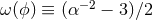
When the coupling  is constant, then Eq. (15*) reduces to the massless version of
Jordan–Fierz–Brans–Dicke theory [82].
is constant, then Eq. (15*) reduces to the massless version of
Jordan–Fierz–Brans–Dicke theory [82].
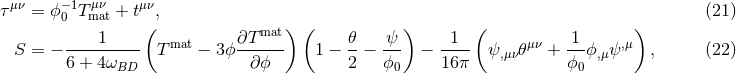
The modified field equations in the Einstein frame are
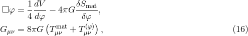
where
is a stress-energy tensor for the scalar field. The matter stress–energy tensor is not constructed from the Einstein-frame metric alone, but by the combination![[ ] (φ) 1 1 ,δ 1 Tμν = --- φ,μφ,ν − --gμνφ,δφ − --gμνV(φ ) (17 ) 4π 2 4](article93x.gif)
 . In the Jordan frame and neglecting the
potential, the modified field equations are [435*]
. In the Jordan frame and neglecting the
potential, the modified field equations are [435*]
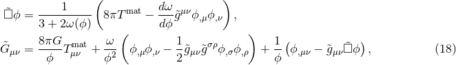
where  is the trace of the matter stress-energy tensor
  constructed from the physical metric
 . The form of the modified field equations in Jordan frame suggest that in the weak-field
limit one may consider scalar-tensor theories as modifying Newton’s gravitational constant via
. The form of the modified field equations in Jordan frame suggest that in the weak-field
limit one may consider scalar-tensor theories as modifying Newton’s gravitational constant via
 .
.
Using the decompositions of Eqs. (3*)-(4*), the field equations of massless Jordan–Fierz–Brans–Dicke theory can be linearized in the Jordan frame to find (see, e.g., [441*])
where
 is the D’Alembertian operator of flat spacetime, we have defined a new metric perturbation
i.e., the metric perturbation in the Einstein frame, with
is the D’Alembertian operator of flat spacetime, we have defined a new metric perturbation
i.e., the metric perturbation in the Einstein frame, with 
 the trace of the metric perturbation
and
the trace of the metric perturbation
and
with cubic remainders in either the metric perturbation or the scalar perturbation. The
quantity  arises in an effective point-particle theory, where the matter action is a
functional of both the Jordan-frame metric and the scalar field. The quantity
arises in an effective point-particle theory, where the matter action is a
functional of both the Jordan-frame metric and the scalar field. The quantity  is a function of
quadratic or higher order in
is a function of
quadratic or higher order in  or
or  . These equations can now be solved given a particular
physical system, as done for quasi-circular binaries in [441*, 374, 336]. Given the above evolution
equations, Jordan–Fierz–Brans–Dicke theory possesses a scalar (spin-0) mode, in addition to the two
transverse-traceless (spin-2) modes of GR, i.e., Jordan–Fierz–Brans–Dicke theory is of Type
. These equations can now be solved given a particular
physical system, as done for quasi-circular binaries in [441*, 374, 336]. Given the above evolution
equations, Jordan–Fierz–Brans–Dicke theory possesses a scalar (spin-0) mode, in addition to the two
transverse-traceless (spin-2) modes of GR, i.e., Jordan–Fierz–Brans–Dicke theory is of Type  in the
 classification [161*, 438*].
Let us now discuss whether scalar-tensor theories satisfy the properties discussed in Section 2.1.
Massless Jordan–Fierz–Brans–Dicke theory agrees with all known experimental tests provided
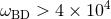 , a bound imposed by the tracking of the Cassini spacecraft through observations of the
Shapiro time delay [73*]. Massive Jordan–Fierz–Brans–Dicke theory has been recently constrained to
, a bound imposed by the tracking of the Cassini spacecraft through observations of the
Shapiro time delay [73*]. Massive Jordan–Fierz–Brans–Dicke theory has been recently constrained to
 and
and  , with
  the mass of the scalar field [348, 20*].
Of course, these bounds are not independent, as when
the mass of the scalar field [348, 20*].
Of course, these bounds are not independent, as when  one recovers the standard
massless constraint, while when
one recovers the standard
massless constraint, while when  ,
,  cannot be bounded as the scalar becomes
non-dynamical. Observations of the Nordtvedt effect with Lunar Laser Ranging observations, as well as
observations of the orbital period derivative of white-dwarf/neutron-star binaries, yield similar
constraints [131*, 132*, 20*, 177*]. Neglecting any homogeneous, cosmological solutions to the scalar-field
evolution equation, it is clear that in the limit
cannot be bounded as the scalar becomes
non-dynamical. Observations of the Nordtvedt effect with Lunar Laser Ranging observations, as well as
observations of the orbital period derivative of white-dwarf/neutron-star binaries, yield similar
constraints [131*, 132*, 20*, 177*]. Neglecting any homogeneous, cosmological solutions to the scalar-field
evolution equation, it is clear that in the limit  one recovers GR, i.e., scalar-tensor theories
have a continuous limit to Einstein’s theory, but see [164*] for caveats for certain spacetimes.
Moreover, [375, 278, 425] have verified that scalar-tensor theories with minimal or non-minimal
coupling in the Jordan frame can be cast in a strongly-hyperbolic form, and thus, they possess a
well-posed initial-value formulation. Therefore, scalar-tensor theories possess both Properties (1) and
(3).
one recovers GR, i.e., scalar-tensor theories
have a continuous limit to Einstein’s theory, but see [164*] for caveats for certain spacetimes.
Moreover, [375, 278, 425] have verified that scalar-tensor theories with minimal or non-minimal
coupling in the Jordan frame can be cast in a strongly-hyperbolic form, and thus, they possess a
well-posed initial-value formulation. Therefore, scalar-tensor theories possess both Properties (1) and
(3).
Scalar-tensor theories also possess Property (2), since they can be derived from the low-energy limit of
certain string theories. The integration of string quantum fluctuations leads to a higher-dimensional string
theoretical action that reduces locally to a field theory similar to a scalar-tensor one [189, 176], the
mapping being  , with
  one of the string moduli fields [133, 134]. Moreover, scalar-tensor
theories can be mapped to
one of the string moduli fields [133, 134]. Moreover, scalar-tensor
theories can be mapped to  theories, where one replaces the Ricci scalar by some functional of
  .
In particular, one can show that
.
In particular, one can show that  theories are equivalent to Brans–Dicke theory with
  , via
the mapping
, via
the mapping  and
and  [104, 396]. For a recent review on this
topic, see [135].
[104, 396]. For a recent review on this
topic, see [135].
Black holes and stars continue to exist in scalar-tensor theories. Stellar configurations are modified from their GR profile [441*, 131*, 214, 215, 410, 132*, 394, 139, 393, 235*], while black holes are not, provided one neglects homogeneous, cosmological solutions to the scalar field evolution equation. Indeed, Hawking [224*, 159*, 222*, 98*, 244*, 363*] has proven that Brans–Dicke black holes that are stationary and the endpoint of gravitational collapse are identical to those of GR. This proof has recently been extended to a general class of scalar-tensor models [398*]. That is, stationary black holes radiate any excess “hair”, i.e., additional degrees of freedom, after gravitational collapse, a result sometimes referred to as the no-hair theorem for black holes in scalar-tensor theories. This result has recently been extended even further to allow for quasi-stationary scenarios in generic scalar-tensor theories through the study of extreme–mass-ratio inspirals [465*] (small black hole in orbit around a much larger one), post-Newtonian comparable-mass inspirals [315*] and numerical simulations of comparable-mass black-hole mergers [230*, 67*].
Damour and Esposito-Farèse [129*, 130*] proposed a different type of scalar-tensor theory, one that can
be defined by the action in Eq. (15*) but with the conformal factor  or the coupling
function
or the coupling
function  , where
  and
and  are constants. When
  one recovers
standard Brans–Dicke theory. When
one recovers
standard Brans–Dicke theory. When  , non-perturbative effects that develop if the gravitational
energy is large enough can force neutron stars to spontaneously acquire a non-trivial scalar field profile, to
spontaneously scalarize. Through this process, a neutron-star binary that initially had no scalar hair in its
early inspiral would acquire it before merger, when the binding energy exceeded some threshold [51*]. Binary
pulsar observations have constrained this theory in the
, non-perturbative effects that develop if the gravitational
energy is large enough can force neutron stars to spontaneously acquire a non-trivial scalar field profile, to
spontaneously scalarize. Through this process, a neutron-star binary that initially had no scalar hair in its
early inspiral would acquire it before merger, when the binding energy exceeded some threshold [51*]. Binary
pulsar observations have constrained this theory in the  space; very roughly speaking
  and
and
 [131, 132, 177]
As for Property (4), scalar tensor theories are not built with the aim of introducing strong-field corrections to GR.3 Instead, they naturally lead to modifications of Einstein’s theory in the weak-field, modifications that dominate in scenarios with sufficiently weak gravitational interactions. Although this might seem strange, it is natural if one considers, for example, one of the key modifications introduced by scalar-tensor theories: the emission of dipolar gravitational radiation. Such dipolar emission dominates over the general relativistic quadrupolar emission for systems in the weak to intermediate field regime, such as in binary pulsars or in the very early inspiral of compact binaries. Therefore, one would expect scalar-tensor theories to be best constrained by experiments or observations of weakly-gravitating systems, as it has recently been explicitly shown in [465*].
2.3.2 Massive graviton theories and Lorentz violation
Massive graviton theories are those in which the gravitational interaction is propagated by a massive gauge
boson, i.e., a graviton with mass  or Compton wavelength
  . Einstein’s theory
predicts massless gravitons and thus gravitational propagation at light speed, but if this were not the case,
then a certain delay would develop between electromagnetic and gravitational signals emitted
simultaneously at the source. Fierz and Pauli [169*] were the first to write down an action for a free massive
graviton, and ever since then, much work has gone into the construction of such models. For a detailed
review, see, e.g., [232].
. Einstein’s theory
predicts massless gravitons and thus gravitational propagation at light speed, but if this were not the case,
then a certain delay would develop between electromagnetic and gravitational signals emitted
simultaneously at the source. Fierz and Pauli [169*] were the first to write down an action for a free massive
graviton, and ever since then, much work has gone into the construction of such models. For a detailed
review, see, e.g., [232].
Gravitational theories with massive gravitons are somewhat well-motivated from a fundamental
physics perspective, and thus, one can say they possess Property (2). Indeed, in loop quantum
cosmology [42, 77], the cosmological extension to loop quantum gravity, the graviton dispersion relation
acquires holonomy corrections during loop quantization that endow the graviton with a mass [78*]
 , with
  the Barbero–Immirzi parameter,
  the area operator, and
  and
and  the total and critical energy density respectively. In string-theory–inspired effective
theories, such as Dvali’s compact, extra-dimensional theory [157], such massive modes also
arise.
the total and critical energy density respectively. In string-theory–inspired effective
theories, such as Dvali’s compact, extra-dimensional theory [157], such massive modes also
arise.
Massive graviton modes also occur in many other modified gravity models. In Rosen’s bimetric theory [365*], for example, photons and gravitons follow null geodesics of different metrics [438*, 435*]. In Visser’s massive graviton theory [424*], the graviton is given a mass at the level of the action through an effective perturbative description of gravity, at the cost of introducing a non-dynamical background metric, i.e., a prior geometry. A recent re-incarnation of this model goes by the name of bigravity, where again two metric tensors are introduced [349*, 346*, 219*, 220*]. In Bekenstein’s Tensor-Vector-Scalar (TeVeS) theory [54], the existence of a scalar and a vector field lead to subluminal gravitational-wave propagation.
Massive graviton theories have a theoretical issue, the van Dam–Veltman–Zakharov (vDVZ)
discontinuity [418, 475], which is associated with Property 1.a, i.e., a GR limit. The problem is that certain
predictions of massive graviton theories do not reduce to those of GR in the  limit. This can be
understood qualitatively by studying how the
limit. This can be
understood qualitatively by studying how the  spin states of the graviton behave in this limit. Two of
them become the two GR helicity states of the massless graviton. Another two become helicity states of a
massless vector that decouples from the tensor perturbations in the
spin states of the graviton behave in this limit. Two of
them become the two GR helicity states of the massless graviton. Another two become helicity states of a
massless vector that decouples from the tensor perturbations in the  limit. However, the last state,
the scalar mode, retains a finite coupling to the trace of the stress-energy tensor in this limit. Therefore,
massive graviton theories in the
limit. However, the last state,
the scalar mode, retains a finite coupling to the trace of the stress-energy tensor in this limit. Therefore,
massive graviton theories in the  limit do not reduce to GR, since the scalar mode does not
decouple.
limit do not reduce to GR, since the scalar mode does not
decouple.
However, the vDVZ discontinuity can be evaded, for example, by carefully including non-linearities.
Vainshtein [413, 269, 140, 45] showed that around any spherically-symmetric source of mass  , there
exists a certain radius
, there
exists a certain radius  , with
  the Schwarzschild radius, where linear theory cannot
be trusted. Since
the Schwarzschild radius, where linear theory cannot
be trusted. Since  as
as  , this implies that there is no radius at which the linear
approximation (and thus vDVZ discontinuity) can be trusted. Of course, to determine then whether massive
graviton theories have a continuous limit to GR, one must include non-linear corrections to the action (see
also an argument by [34]), which are more difficult to uniquely predict from fundamental theory.
Recently, there has been much activity in the development of new, non-linear massive gravity
theories [60*, 136*, 211, 61, 137, 138].
, this implies that there is no radius at which the linear
approximation (and thus vDVZ discontinuity) can be trusted. Of course, to determine then whether massive
graviton theories have a continuous limit to GR, one must include non-linear corrections to the action (see
also an argument by [34]), which are more difficult to uniquely predict from fundamental theory.
Recently, there has been much activity in the development of new, non-linear massive gravity
theories [60*, 136*, 211, 61, 137, 138].
Lacking a particular action for massive graviton theories that modifies the strong-field regime and is free of non-linear and radiatively-induced ghosts, it is difficult to ascertain many of its properties, but this does not prevent us from considering certain phenomenological effects. If the graviton is truly massive, whatever the action may be, two main modifications to Einstein’s theory will be introduced:
- Modification to Newton’s laws;
- Modification to gravitational wave propagation.
Modifications of class (i) correspond to the replacement of the Newtonian potential by a
Yukawa type potential (in the non-radiative, near-zone of any body of mass  ):
):
 , where
  is the distance to the body [437*]. Tests of such a Yukawa
interaction have been proposed through observations of bound clusters, tidal interactions between
galaxies [200] and weak gravitational lensing [106], but such tests are model dependent.
is the distance to the body [437*]. Tests of such a Yukawa
interaction have been proposed through observations of bound clusters, tidal interactions between
galaxies [200] and weak gravitational lensing [106], but such tests are model dependent.
Modifications of class (ii) are in the form of a non-zero graviton mass that induces a modified gravitational-wave dispersion relation. Such a modification to the dispersion relation was originally parameterized via [437*]
where
 and
and  are the speed and mass of the graviton, while
  is its energy, usually associated to
its frequency via the quantum mechanical relation
is its energy, usually associated to
its frequency via the quantum mechanical relation  . This modified dispersion relation is inspired
by special relativity, a more general version of which, inspired by quantum gravitational theories, is [316*]
where
. This modified dispersion relation is inspired
by special relativity, a more general version of which, inspired by quantum gravitational theories, is [316*]
where 
 is now a parameter that depends on the theory and
  represents deviations from light-speed
propagation. For example, in Rosen’s bimetric theory [365], the graviton does not travel at the speed of
light, but at some other speed partially determined by the prior geometry. In metric theories of gravity,
represents deviations from light-speed
propagation. For example, in Rosen’s bimetric theory [365], the graviton does not travel at the speed of
light, but at some other speed partially determined by the prior geometry. In metric theories of gravity,
 , where
  is some amplitude that depends on the metric theory (see discussion in [316*]).
Either modification to the dispersion relation has the net effect of slowing gravitons down, such that there is
a difference in the time of arrival of photons and gravitons. Moreover, such an energy-dependent
dispersion relation would also affect the accumulated gravitational-wave phase observed by
gravitational-wave detectors, as we discuss in Section 5. Given these modifications to the dispersion
relation, one would expect the generation of gravitational waves to also be greatly affected in such
theories, but again, lacking a particular healthy action to consider, this topic remains today mostly
unexplored.
is some amplitude that depends on the metric theory (see discussion in [316*]).
Either modification to the dispersion relation has the net effect of slowing gravitons down, such that there is
a difference in the time of arrival of photons and gravitons. Moreover, such an energy-dependent
dispersion relation would also affect the accumulated gravitational-wave phase observed by
gravitational-wave detectors, as we discuss in Section 5. Given these modifications to the dispersion
relation, one would expect the generation of gravitational waves to also be greatly affected in such
theories, but again, lacking a particular healthy action to consider, this topic remains today mostly
unexplored.
From the structure of the above phenomenological modifications, it is clear that GR can be recovered in
the  limit, avoiding the vDVZ issue altogether by construction. Such phenomenological
modifications have been constrained by several types of experiments and observations. Using the
modification to Newton’s third law and precise observations of the motion of the inner planets of the solar
system together with Kepler’s third law, [437*] found a bound of
limit, avoiding the vDVZ issue altogether by construction. Such phenomenological
modifications have been constrained by several types of experiments and observations. Using the
modification to Newton’s third law and precise observations of the motion of the inner planets of the solar
system together with Kepler’s third law, [437*] found a bound of  . Such a constraint is
purely static, as it does not sample the radiative sector of the theory. Dynamical constraints, however, do
exist: through observations of the decay of the orbital period of binary pulsars, [174*] found a bound of
. Such a constraint is
purely static, as it does not sample the radiative sector of the theory. Dynamical constraints, however, do
exist: through observations of the decay of the orbital period of binary pulsars, [174*] found a bound of
 ;4
by investigating the stability of Schwarzschild and Kerr black holes, [88*] placed the constraint
;4
by investigating the stability of Schwarzschild and Kerr black holes, [88*] placed the constraint
 in Fierz–Pauli theory [169*]. New constraints that use gravitational waves have been
proposed, including measuring a difference in time of arrival of electromagnetic and gravitational
waves [126*, 266], as well as direct observation of gravitational waves emitted by binary pulsars (see
Section 5).
in Fierz–Pauli theory [169*]. New constraints that use gravitational waves have been
proposed, including measuring a difference in time of arrival of electromagnetic and gravitational
waves [126*, 266], as well as direct observation of gravitational waves emitted by binary pulsars (see
Section 5).
Although massive gravity theories unavoidably lead to a modification to the graviton dispersion relation, the converse is not necessarily true. A modification of the dispersion relation is usually accompanied by a modification to either the Lorentz group or its action in real or momentum space. Such Lorentz-violating effects are commonly found in quantum gravitational theories, including loop quantum gravity [78] and string theory [107, 403], as well as other effective models [58, 59]. In doubly-special relativity [26, 300, 27, 28], the graviton dispersion relation is modified at high energies by modifying the law of transformation of inertial observers. Modified graviton dispersion relations have also been shown to arise in generic extra-dimensional models [381], in Hořava–Lifshitz theory [233, 234*, 412, 76] and in theories with non-commutative geometries [186, 187, 188]. None of these theories necessarily requires a massive graviton, but rather the modification to the dispersion relation is introduced due to Lorentz-violating effects.
One might be concerned that the mass of the graviton and subsequent modifications to the graviton dispersion relation should be suppressed by the Planck scale. However, Collins, et al. [111, 110] have suggested that Lorentz violations in perturbative quantum field theories could be dramatically enhanced when one regularizes and renormalizes them. This is because terms that vanish upon renormalization due to Lorentz invariance do not vanish in Lorentz-violating theories, thus leading to an enhancement [185]. Whether such an enhancement is truly present cannot currently be ascertained.
2.3.3 Modified quadratic gravity
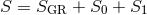
Modified quadratic gravity is a family of models first discussed in the context of black holes and gravitational waves in [473*, 447*]. The 4-dimensional action is given by
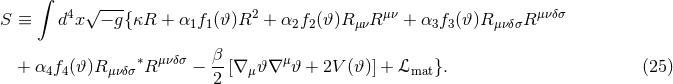
The quantity  is the dual to the Riemann tensor. The quantity
  is the
external matter Lagrangian, while
is the
external matter Lagrangian, while  are functionals of the field
  , with
  coupling
constants and
coupling
constants and  . Clearly, the two terms second to last in Eq. (25) represent
a canonical kinetic energy term and a potential. At this stage, one might be tempted to set
. Clearly, the two terms second to last in Eq. (25) represent
a canonical kinetic energy term and a potential. At this stage, one might be tempted to set
 or the
  via a rescaling of the scalar field functional, but we shall not do so
here.
via a rescaling of the scalar field functional, but we shall not do so
here.
The action in Eq. (25) is well-motivated from fundamental theories, as it contains all possible quadratic,
algebraic curvature scalars with running (i.e., non-constant) couplings. The only restriction here is that all
quadratic terms are assumed to couple to the same field, which need not be the case. For example, in string
theory some terms might couple to the dilaton (a scalar field), while others couple to the axion (a pseudo
scalar field). Nevertheless, one can recover well-known and motivated modified gravity theories in simple
cases. For example, dynamical Chern–Simons modified gravity [17*] is recovered when  and
all other
and
all other  . Einstein-Dilaton-Gauss–Bonnet gravity [343*] is obtained when
  and
and
 .5
Both theories unavoidably arise as low-energy expansions of heterotic string theory [203*, 204*, 12*, 89*]. As
such, modified quadratic gravity theories should be treated as a class of effective field theories. Moreover,
dynamical Chern–Simons gravity also arises in loop quantum gravity [43, 366] when the Barbero–Immirzi
parameter is promoted to a field in the presence of fermions [41*, 16, 406*, 311*, 192*].
.5
Both theories unavoidably arise as low-energy expansions of heterotic string theory [203*, 204*, 12*, 89*]. As
such, modified quadratic gravity theories should be treated as a class of effective field theories. Moreover,
dynamical Chern–Simons gravity also arises in loop quantum gravity [43, 366] when the Barbero–Immirzi
parameter is promoted to a field in the presence of fermions [41*, 16, 406*, 311*, 192*].
One should make a clean and clear distinction between the theory defined by the action of
Eq. (25) and that of  theories. The latter are defined as functionals of the Ricci scalar only,
while Eq. (25) contains terms proportional to the Ricci tensor and Riemann tensor squared.
One could think of the subclass of
theories. The latter are defined as functionals of the Ricci scalar only,
while Eq. (25) contains terms proportional to the Ricci tensor and Riemann tensor squared.
One could think of the subclass of  theories with
  as the limit of modified
quadratic gravity with only
as the limit of modified
quadratic gravity with only  and
and  . In that very special case, one can map
quadratic gravity theories and
. In that very special case, one can map
quadratic gravity theories and  gravity to a scalar-tensor theory. Another important
distinction is that
gravity to a scalar-tensor theory. Another important
distinction is that  theories are usually treated as exact, while the action presented above
is to be interpreted as an effective theory [89*] truncated to quadratic order in the curvature
in a low-energy expansion of a more fundamental theory. This implies that there are cubic,
quartic, etc. terms in the Riemann tensor that are not included in Eq. (25) and that presumably
depend on higher powers of
theories are usually treated as exact, while the action presented above
is to be interpreted as an effective theory [89*] truncated to quadratic order in the curvature
in a low-energy expansion of a more fundamental theory. This implies that there are cubic,
quartic, etc. terms in the Riemann tensor that are not included in Eq. (25) and that presumably
depend on higher powers of  . Thus, when studying such an effective theory one should also
order-reduce the field equations and treat all quantities that depend on
. Thus, when studying such an effective theory one should also
order-reduce the field equations and treat all quantities that depend on  perturbatively,
the small-coupling approximation. One can show that such an order reduction removes any
additional polarization modes in propagating metric perturbations [390*, 400*] that naturally arise in
perturbatively,
the small-coupling approximation. One can show that such an order reduction removes any
additional polarization modes in propagating metric perturbations [390*, 400*] that naturally arise in
 theories. In analogy to the treatment of the Ostrogradski instability in Section 2.1, one
would also expect that order-reduction would lead to a theory with a well-posed initial-value
formulation.
theories. In analogy to the treatment of the Ostrogradski instability in Section 2.1, one
would also expect that order-reduction would lead to a theory with a well-posed initial-value
formulation.
This family of theories is usually simplified by making the assumption that coupling functions  admit a Taylor expansion:
  for small
  , where
  and
and  are
constants and
are
constants and  is assumed to vanish at asymptotic spatial infinity. Reabsorbing
  into the coupling
constants
into the coupling
constants  and
and  into the constants
  , Eq. (25) becomes
 with
with
Here,  is the Einstein–Hilbert plus matter action, while
  and
and  are corrections. The former
is decoupled from
are corrections. The former
is decoupled from  , where the omitted term proportional to
  does not affect the classical field
equations since it is topological, i.e., it can be rewritten as the total
does not affect the classical field
equations since it is topological, i.e., it can be rewritten as the total  -divergence of some
 -current. Similarly, if the
  were chosen to reconstruct the Gauss–Bonnet invariant,
 , then this combination would also be topological and not affect
the classical field equations. On the other hand,
, then this combination would also be topological and not affect
the classical field equations. On the other hand,  is a modification to GR with a direct
(non-minimal) coupling to
is a modification to GR with a direct
(non-minimal) coupling to  , such that as the field goes to zero, the modified theory reduces to
GR.
, such that as the field goes to zero, the modified theory reduces to
GR.
Another restriction one usually makes to simplify modified gravity theories is to neglect the  terms
and only consider the
terms
and only consider the  modification, the restricted modified quadratic gravity. The
  terms
represent corrections that are non-dynamical. The term proportional to
terms
represent corrections that are non-dynamical. The term proportional to  resembles a certain class
of
resembles a certain class
of  theories. As such, it can be mapped to a scalar-tensor theory with a complicated
potential, which has been heavily constrained by torsion-balance Eöt-Wash experiments to
theories. As such, it can be mapped to a scalar-tensor theory with a complicated
potential, which has been heavily constrained by torsion-balance Eöt-Wash experiments to
 [237, 259*, 62]. Moreover, these theories have a fixed coupling constant that does not
run with energy or scale. In restricted modified gravity, the scalar field is effectively forcing the running of
the coupling.
[237, 259*, 62]. Moreover, these theories have a fixed coupling constant that does not
run with energy or scale. In restricted modified gravity, the scalar field is effectively forcing the running of
the coupling.
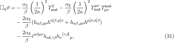
Then, let us concentrate on restricted modified quadratic gravity and drop the superscript in  . The
modified field equations are
. The
modified field equations are
where we have defined
The  stress-energy tensor is
![[ 1 ( )] T(μ𝜗ν)= β (∇ μ𝜗 )(∇ ν𝜗 ) −--gμν ∇ δ𝜗∇ δ𝜗 − 2V (𝜗) . (29 ) 2](article228x.gif)

Notice that unlike traditional scalar-tensor theories, the scalar field is here sourced by the geometry and not by the matter distribution. This directly implies that black holes in such theories are likely to be hairy.
From the structure of the above equations, it should be clear that the dynamics of  guarantee that
the modified field equations are covariantly conserved exactly. That is, one can easily verify that the
covariant divergence of Eq. (27) identically vanishes upon imposition of Eq. (30). Such a result had to be
so, as the action is diffeomorphism invariant. If one neglected the kinetic and potential energies of
guarantee that
the modified field equations are covariantly conserved exactly. That is, one can easily verify that the
covariant divergence of Eq. (27) identically vanishes upon imposition of Eq. (30). Such a result had to be
so, as the action is diffeomorphism invariant. If one neglected the kinetic and potential energies of  in
the action, as was originally done in [245*], the theory would possess preferred-frame effects and would not
be covariantly conserved. Moreover, such a theory requires an additional constraint, i.e., the right-hand
side of (30) would have to vanish, which is an unphysical consequence of treating
in
the action, as was originally done in [245*], the theory would possess preferred-frame effects and would not
be covariantly conserved. Moreover, such a theory requires an additional constraint, i.e., the right-hand
side of (30) would have to vanish, which is an unphysical consequence of treating  as prior
structure [470*, 207*].
as prior
structure [470*, 207*].
One last simplification that is usually made when studying modified quadratic gravity theories is to
ignore the potential  , i.e., set
  . This potential can in principle be non-zero, for example if
one wishes to endow
. This potential can in principle be non-zero, for example if
one wishes to endow  with a mass or if one wishes to introduce a cosine driving term, like that for axions
in field and string theory. However, reasons exist to restrict the functional form of such a potential. First, a
mass for
with a mass or if one wishes to introduce a cosine driving term, like that for axions
in field and string theory. However, reasons exist to restrict the functional form of such a potential. First, a
mass for  will modify the evolution of any gravitational degree of freedom only if this mass is
comparable to the inverse length scale of the problem under consideration (such as a binary system). This
could be possible if there is an incredibly large number of fields with different masses in the theory, such as
perhaps in the string axiverse picture [40, 268, 303]. However, in that picture the moduli fields are
endowed with a mass due to shift-symmetry breaking by non-perturbative effects; such masses are
not expected to be comparable to the inverse length scale of binary systems. Second, no mass
term may appear in a theory with a shift symmetry, i.e., invariance under the transformation
will modify the evolution of any gravitational degree of freedom only if this mass is
comparable to the inverse length scale of the problem under consideration (such as a binary system). This
could be possible if there is an incredibly large number of fields with different masses in the theory, such as
perhaps in the string axiverse picture [40, 268, 303]. However, in that picture the moduli fields are
endowed with a mass due to shift-symmetry breaking by non-perturbative effects; such masses are
not expected to be comparable to the inverse length scale of binary systems. Second, no mass
term may appear in a theory with a shift symmetry, i.e., invariance under the transformation
 . Such symmetries are common in four-dimensional, low-energy, effective string
theories [79, 204*, 203, 92, 89], such as dynamical Chern–Simons and Einstein-Dilaton-Gauss–Bonnet
theory. Similar considerations apply to other more complicated potentials, such as a cosine
term.
. Such symmetries are common in four-dimensional, low-energy, effective string
theories [79, 204*, 203, 92, 89], such as dynamical Chern–Simons and Einstein-Dilaton-Gauss–Bonnet
theory. Similar considerations apply to other more complicated potentials, such as a cosine
term.
Given these field equations, one can linearize them about Minkowski space to find evolution equations for the perturbation in the small-coupling approximation. Doing so, one finds [447*]
where we have order-reduced the theory where possible and used the harmonic gauge condition (which is
preserved in this class of theories [390*, 400*]). The corresponding equation for the metric perturbation is
rather lengthy and can be found in Eqs. (17) – (24) in [447*]. Since these theories are to be considered
effective, working always to leading order in  , one can show that they are perturbatively of type
  in
the
in
the  classification [161*], i.e., in the far zone, the only propagating modes that survive are the two
transverse-traceless (spin-2) metric perturbations [390*]. However, in the strong-field region it is possible
that additional modes are excited, although they decay rapidly as they propagate to future null
infinity.
classification [161*], i.e., in the far zone, the only propagating modes that survive are the two
transverse-traceless (spin-2) metric perturbations [390*]. However, in the strong-field region it is possible
that additional modes are excited, although they decay rapidly as they propagate to future null
infinity.
Lastly, let us discuss what is known about whether modified quadratic gravities satisfy the
requirements discussed in Section 2.1. As it should be clear from the action itself, this modified
gravity theory satisfies the fundamental requirement, i.e., passing all precision tests, provided the
couplings  are sufficiently small. This is because such theories have a continuous limit to GR as
 .6
Dynamical Chern–Simons gravity is constrained only weakly at the moment,
.6
Dynamical Chern–Simons gravity is constrained only weakly at the moment,  , where
 , only through observations of Lense–Thirring precession in the solar system [19*]. The
Einstein-Dilaton-Gauss–Bonnet gravity coupling constant
, only through observations of Lense–Thirring precession in the solar system [19*]. The
Einstein-Dilaton-Gauss–Bonnet gravity coupling constant  , on the other hand, has been
constrained by several experiments: solar system observations of the Shapiro time delay with the Cassini
spacecraft placed the bound
, on the other hand, has been
constrained by several experiments: solar system observations of the Shapiro time delay with the Cassini
spacecraft placed the bound  [73*, 29]; the requirement that neutron stars still
exist in this theory placed the constraint
[73*, 29]; the requirement that neutron stars still
exist in this theory placed the constraint  [342*], with the details depending
somewhat on the central density of the neutron star; observations of the rate of change of the
orbital period in the low-mass X-ray binary A0620–00 [358, 255*] has led to the constraint
[342*], with the details depending
somewhat on the central density of the neutron star; observations of the rate of change of the
orbital period in the low-mass X-ray binary A0620–00 [358, 255*] has led to the constraint
 [445].
However, not all sub-properties of the fundamental requirement are known to be satisfied.
One can show that certain members of modified quadratic gravity possess known solutions
and these are stable, at least in the small-coupling approximation. For example, in dynamical
Chern–Simons gravity, spherically-symmetric vacuum solutions are given by the Schwarzschild
metric with constant  to all orders in
  [245*, 470*]. Such a solution is stable to small
perturbations [319, 190*], as also are non-spinning black holes and branes in anti de Sitter space [144].
On the other hand, spinning solutions continue to be elusive, with approximate solutions in
the slow-rotation/small-coupling limit known both for black holes [466*, 272*, 345*, 455*] and
stars [19*, 342*]; nothing is currently known about the stability of these spinning solutions. In
Einstein-Dilaton-Gauss–Bonnet theory even spherically-symmetric solutions are modified [473*, 345*] and
these are stable to axial perturbations [343*].
[245*, 470*]. Such a solution is stable to small
perturbations [319, 190*], as also are non-spinning black holes and branes in anti de Sitter space [144].
On the other hand, spinning solutions continue to be elusive, with approximate solutions in
the slow-rotation/small-coupling limit known both for black holes [466*, 272*, 345*, 455*] and
stars [19*, 342*]; nothing is currently known about the stability of these spinning solutions. In
Einstein-Dilaton-Gauss–Bonnet theory even spherically-symmetric solutions are modified [473*, 345*] and
these are stable to axial perturbations [343*].
The study of modified quadratic gravity theories as effective theories is valid provided one is sufficiently
far from its cut-off scale, i.e., the scale beyond which higher-order curvature terms cannot be neglected
anymore. One can estimate the magnitude of this scale by studying the size of loop corrections to the
quadratic curvature terms in the action due to  -point interactions [455*]. Simple counting requires that
the number of scalar and graviton propagators,
-point interactions [455*]. Simple counting requires that
the number of scalar and graviton propagators,  and
and  , satisfy the following relation in terms of the
number of vertices
, satisfy the following relation in terms of the
number of vertices  :
:

 , with
  the Planck mass and
  the energy scale introduced by dimensional arguments. The cut-off scale above which the theory cannot be
treated as an effective one can be approximated as the value of
the energy scale introduced by dimensional arguments. The cut-off scale above which the theory cannot be
treated as an effective one can be approximated as the value of  at which the suppression factor becomes
equal to unity:
This cut-off scale automatically places a constraint on the magnitude of
at which the suppression factor becomes
equal to unity:
This cut-off scale automatically places a constraint on the magnitude of 
 above which higher-curvature
corrections must be included. Setting the largest value of
above which higher-curvature
corrections must be included. Setting the largest value of  to be equal to
  ), thus saturating
bounds from table-top experiments [259*], and solving for
), thus saturating
bounds from table-top experiments [259*], and solving for  , we find
Current solar system bounds on
, we find
Current solar system bounds on 
 already require the coupling constant to be smaller than
  ,
thus justifying the treatment of these theories as effective models.
,
thus justifying the treatment of these theories as effective models.
As for the other requirements discussed in Section 2.1, it is clear that modified quadratic gravity is
well-motivated from fundamental theory, but it is not clear at all whether it has a well-posed initial-value
formulation. From an effective point of view, a perturbative treatment in  naturally leads to stable
solutions and a well-posed initial-value problem, but this is probably not the case when it is treated as an
exact theory. In fact, if one were to treat such a theory as exact (to all orders in
naturally leads to stable
solutions and a well-posed initial-value problem, but this is probably not the case when it is treated as an
exact theory. In fact, if one were to treat such a theory as exact (to all orders in  ), then the evolution
system would likely not be hyperbolic, as higher-than-second time derivatives now drive the
evolution. Although no proof exists, it is likely that such an exact theory is not well-posed as an
initial-value problem. Notice, however, that this says nothing about the fundamental theories that
modified quadratic gravity derives from. This is because even if the truncated theory were
ill posed, higher-order corrections that are neglected in the truncated version could restore
well-posedness.
), then the evolution
system would likely not be hyperbolic, as higher-than-second time derivatives now drive the
evolution. Although no proof exists, it is likely that such an exact theory is not well-posed as an
initial-value problem. Notice, however, that this says nothing about the fundamental theories that
modified quadratic gravity derives from. This is because even if the truncated theory were
ill posed, higher-order corrections that are neglected in the truncated version could restore
well-posedness.
As for the last requirement (that the theory modifies the strong field), modified quadratic theories are ideal in this respect. This is because they introduce corrections to the action that depend on higher powers of the curvature. In the strong-field, such higher powers could potentially become non-negligible relative to the Einstein–Hilbert action. Moreover, since the curvature scales inversely with the mass of the objects under consideration, one expects the largest deviations in systems with small total mass, such as stellar-mass black-hole mergers. On the other hand, deviations from GR should be small for small compact objects spiraling into a supermassive black hole, since here the spacetime curvature is dominated by the large object, and thus it is small, as discussed in [390*].
2.3.4 Variable G theories and large extra dimensions
Variable  theories are defined as those where Newton’s gravitational constant is promoted
to a spacetime function. Such a modification breaks the principle of equivalence (see [438*])
because the laws of physics now become local position dependent. In turn, this implies that
experimental results now depend on the spacetime position of the laboratory frame at the time of the
experiment.
theories are defined as those where Newton’s gravitational constant is promoted
to a spacetime function. Such a modification breaks the principle of equivalence (see [438*])
because the laws of physics now become local position dependent. In turn, this implies that
experimental results now depend on the spacetime position of the laboratory frame at the time of the
experiment.
Many known alternative theories that violate the principle of equivalence, and in particular, the strong
equivalence principle, predict a varying gravitational constant. A classic example is scalar-tensor
theory [435], which, as explained in Section 2.3.1, modifies the gravitational sector of the action
by multiplying the Ricci scalar by a scalar field (in the Jordan frame). In such theories, one
can effectively think of the scalar as promoting the coupling between gravity and matter to a
field-dependent quantity  , thus violating local position invariance when
  varies. Another
example are bimetric theories, such as that of Lightman–Lee [293], where the gravitational
constant becomes time-dependent even in the absence of matter, due to possibly time-dependent
cosmological evolution of the prior geometry. A final example are higher-dimensional, brane-world
scenarios, where enhanced Hawking radiation inexorably leads to a time-varying effective 4D
gravitational constant [141], whose rate of change depends on the curvature radius of extra
dimensions [255*].
varies. Another
example are bimetric theories, such as that of Lightman–Lee [293], where the gravitational
constant becomes time-dependent even in the absence of matter, due to possibly time-dependent
cosmological evolution of the prior geometry. A final example are higher-dimensional, brane-world
scenarios, where enhanced Hawking radiation inexorably leads to a time-varying effective 4D
gravitational constant [141], whose rate of change depends on the curvature radius of extra
dimensions [255*].
One can also construct  -type actions that introduce variability to Newton’s constant. For
example, consider the
-type actions that introduce variability to Newton’s constant. For
example, consider the  model [180*]
![∫ [ ( ) ] 4 √ --- R S = d x − gκR 1 + α0ln --- + Smat, (35 ) R0](article277x.gif)
 ,
,  is a coupling constant and
  is a curvature scale. This action is motivated
by certain renormalization group flow arguments [180*]. The field equations are
is a curvature scale. This action is motivated
by certain renormalization group flow arguments [180*]. The field equations are

where we have defined the new constant
Clearly, the new coupling constant![[ α0 ( R ) ] ¯κ := κ 1 + ---ln --- . (37 ) κ R0](article282x.gif)
 depends on the curvature scale involved in the problem, and thus,
on the geometry, forcing
depends on the curvature scale involved in the problem, and thus,
on the geometry, forcing  to run to zero in the ultraviolet limit.
An important point to address is whether variable  theories can lead to modifications to a vacuum
spacetime, such as a black-hole–binary inspiral. In Einstein’s theory,
theories can lead to modifications to a vacuum
spacetime, such as a black-hole–binary inspiral. In Einstein’s theory,  appears as the coupling constant
between geometry, encoded by the Einstein tensor
appears as the coupling constant
between geometry, encoded by the Einstein tensor  , and matter, encoded by the stress energy tensor
 . When considering vacuum spacetimes,
  and one might naively conclude that a variable
 would not introduce any modification to such spacetimes. In fact, this is the case in scalar-tensor
theories (without homogeneous, cosmological solutions to the scalar field equation), where the no-hair
theorem establishes that black-hole solutions are not modified. On the other hand, scalar-tensor theories
with a cosmological, homogeneous scalar field solution can violate the no-hair theorem, endowing black
holes with time-dependent hair, which in turn would introduce variability into
would not introduce any modification to such spacetimes. In fact, this is the case in scalar-tensor
theories (without homogeneous, cosmological solutions to the scalar field equation), where the no-hair
theorem establishes that black-hole solutions are not modified. On the other hand, scalar-tensor theories
with a cosmological, homogeneous scalar field solution can violate the no-hair theorem, endowing black
holes with time-dependent hair, which in turn would introduce variability into  even in vacuum
spacetimes [246*, 236, 67*].
even in vacuum
spacetimes [246*, 236, 67*].
In general, Newton’s constant plays a much more fundamental role than merely a coupling constant: it
defines the relationship between energy and length. For example, for the vacuum Schwarzschild solution,
 establishes the relationship between the radius
  of the black hole and the rest-mass energy
  of
the spacetime via
of
the spacetime via  . Similarly, in a black-hole–binary spacetime, each black hole introduces an
energy scale into the problem that is quantified by a specification of Newton’s constant. Therefore, one can
treat variable
. Similarly, in a black-hole–binary spacetime, each black hole introduces an
energy scale into the problem that is quantified by a specification of Newton’s constant. Therefore, one can
treat variable  modifications as induced by some effective theory that modifies the mapping between the
curvature scale and the energy scale of the problem, as is done for example in theories with extra
dimensions.
modifications as induced by some effective theory that modifies the mapping between the
curvature scale and the energy scale of the problem, as is done for example in theories with extra
dimensions.
An explicit example of this idea is realized in braneworld models. Superstring theory suggests that physics should be described by 4 large dimensions, plus another 6 that are compactified and very small [354, 355*]. The size of these extra dimensions is greatly constrained by particle theory experiments. However, braneworld models, where a certain higher-dimensional membrane is embedded in a higher-dimensional bulk spacetime, can evade this constraint as only gravitons can interact with the bulk. The ADD model [32, 33] is a particular example of such a braneworld, where the bulk is flat and compact and the brane is tensionless with ordinary fields localized on it. Since gravitational-wave experiments have not yet constrained deviations from Einstein’s theory in the strong field, the size of these extra dimensions is constrained to micrometer scales only by table-top experiments [259, 7*].
What is relevant to gravitational-wave experiments is that in many of these braneworld models black
holes may not remain static [163, 405]. The argument goes roughly as follows: a five-dimensional black hole
is dual to a four-dimensional one with conformal fields on it by the ADS/CFT conjecture [301, 9], but since
the latter must evolve via Hawking radiation, the black hole must be losing mass. The Hawking mass
loss rate is here enhanced by the large number of degrees of freedom in the conformal field
theory, leading to an effective modification to Newton’s laws and to the emission of gravitational
radiation. Effectively, one can think of the black-hole mass loss as due to the black hole being
stretched away from the brane into the bulk due to a universal acceleration, that essentially
reduces the size of the brane-localized black hole. For black-hole binaries, one can then draw
an analogy between this induced time dependence in the black-hole mass and a variable  theory, where Newton’s constant decays due to the presence of black holes. Of course, this is only
analogy, since large extra dimensions would not predict a time-evolving mass in neutron-star
binaries.
theory, where Newton’s constant decays due to the presence of black holes. Of course, this is only
analogy, since large extra dimensions would not predict a time-evolving mass in neutron-star
binaries.
Recently, however, Figueras et al. [170, 172, 171] numerically found stable solutions that do not require a radiation component. If such solutions were the ones realized in nature as a result of gravitational collapse on the brane, then the black hole mass would be time independent, up to quantum correction due to Hawking evaporation, a negligible effect for realistic astrophysical systems. Unfortunately, we currently lack numerical simulations of the dynamics of gravitational collapse in such scenarios.
Many experiments have been carried out to measure possible deviations from a constant
 value, and they can broadly be classified into two groups: (a) those that search for the
present or nearly present rate of variation (at redshifts close to zero); (b) those that search for
secular variations over long time periods (at very large redshifts). Examples of experiments
or observations of the first class include planetary radar ranging [350], surface temperature
observations of low-redshift millisecond pulsars [249, 362], lunar ranging observations [442] and
pulsar timing observations [260, 143], the latter two being the most stringent. Examples of
experiments of the second class include the evolution of the sun [208] and Big-Bang Nucleosynthesis
(BBN) calculations [119, 47], again with the latter being more stringent. For either class, the
strongest constraints are about
value, and they can broadly be classified into two groups: (a) those that search for the
present or nearly present rate of variation (at redshifts close to zero); (b) those that search for
secular variations over long time periods (at very large redshifts). Examples of experiments
or observations of the first class include planetary radar ranging [350], surface temperature
observations of low-redshift millisecond pulsars [249, 362], lunar ranging observations [442] and
pulsar timing observations [260, 143], the latter two being the most stringent. Examples of
experiments of the second class include the evolution of the sun [208] and Big-Bang Nucleosynthesis
(BBN) calculations [119, 47], again with the latter being more stringent. For either class, the
strongest constraints are about 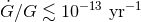 , varying somewhat from experiment to
experiment.
, varying somewhat from experiment to
experiment.
Lacking a particularly compelling action to describe variable  theories, one is usually left
with a phenomenological model of how such a modification to Einstein’s theory would impact
gravitational waves. Given that the part of the waveform that detectors are most sensitive to is
the gravitational wave phase, one can model the effect of variable
theories, one is usually left
with a phenomenological model of how such a modification to Einstein’s theory would impact
gravitational waves. Given that the part of the waveform that detectors are most sensitive to is
the gravitational wave phase, one can model the effect of variable  theories by studying
how the rate of change of its frequency would be modified. Assuming a Taylor expansion for
Newton’s constant one can derive the modification to the evolution equation for the gravitational
wave frequency, given whichever physical scenario one is considering. Solving such an evolution
equation then leads to a modification in the accumulated gravitational-wave phase observed at
detectors on Earth. In Section 5 we will provide an explicit example of this for a compact binary
system.
theories by studying
how the rate of change of its frequency would be modified. Assuming a Taylor expansion for
Newton’s constant one can derive the modification to the evolution equation for the gravitational
wave frequency, given whichever physical scenario one is considering. Solving such an evolution
equation then leads to a modification in the accumulated gravitational-wave phase observed at
detectors on Earth. In Section 5 we will provide an explicit example of this for a compact binary
system.
Let us discuss whether such theories satisfy the criteria defined in Section 2.1. The fundamental
property can be satisfied if the rate of change of Newton’s constant is small enough, as variable  theories
usually have a continuous limit to GR (as all derivatives of
theories
usually have a continuous limit to GR (as all derivatives of  go to zero). Whether variable
  theories
are well-motivated from fundamental physics (Property 2) depends somewhat on the particular effective
model or action that one considers. But in general, Property 2 is usually satisfied, considering that such
variability naturally arises in theories with extra dimensions, and the latter are also natural in all string
theories. However, variable
theories
are well-motivated from fundamental physics (Property 2) depends somewhat on the particular effective
model or action that one considers. But in general, Property 2 is usually satisfied, considering that such
variability naturally arises in theories with extra dimensions, and the latter are also natural in all string
theories. However, variable  theories usually fail at introducing modifications in the strong-field region.
Usually, such variability is parameterized as a Taylor expansion about some initial point with constant
coefficients. That is, the variability of
theories usually fail at introducing modifications in the strong-field region.
Usually, such variability is parameterized as a Taylor expansion about some initial point with constant
coefficients. That is, the variability of  is not usually constructed so as to become stronger closer to
merger.
is not usually constructed so as to become stronger closer to
merger.
The well-posed property and the sub-properties of the fundamental property depend somewhat
on the particular effective theory used to describe varying  modifications. In the
  case, one can impose restrictions on the functional form
  such that no ghosts (
 )
or instabilities (
)
or instabilities ( ) arise [180]. This, of course, does not guarantee that this (or any
other such) theory is well posed. A much more detailed analysis would be required to prove
well-posedness of the class of theories that lead to a variable Newton’s constant, but such is currently
lacking.
) arise [180]. This, of course, does not guarantee that this (or any
other such) theory is well posed. A much more detailed analysis would be required to prove
well-posedness of the class of theories that lead to a variable Newton’s constant, but such is currently
lacking.
2.3.5 Non-commutative geometry
Non-commutative geometry is a gravitational theory that generalizes the continuum Riemannian manifold of Einstein’s theory with the product of it with a tiny, discrete, finite non-commutative space, composed of only two points. Although the non-commutative space has zero spacetime dimension, as the product manifold remains four dimensional, its internal dimensions are 6 to account for Weyl and chiral fermions. This space is discrete to avoid the infinite tower of massive particles that would otherwise be generated, as in string theory. Through this construction, one can recover the standard model of elementary particles, while accounting for all (elementary particle) experimental data to date. Of course, the simple non-commutative space described above is expected to be replaced by a more complex model at Planckian energies. Thus, one is expected to treat such non-commutative geometry models as effective theories. Essentially nothing is currently known about the full non-commutative theory of which the theories described in this section are an effective low-energy limit.
Before proceeding with an action-principle description of non-commutative geometry theories, we must distinguish between the spectral geometry approach championed by Connes [114], and Moyal-type non-commutative geometries [389, 206, 322]. In the former, the manifold is promoted to a non-commutative object through the product of a Riemann manifold with a non-commutative space. In the latter, instead, a non-trivial set of commutation relations is imposed between operators corresponding to position. These two theories are in principle unrelated. In this review, we will concentrate only on the former, as it is the only type of non-commutative GR extension that has been studied in the context of gravitational-wave theory.
The effective action for spectral non-commutative geometry theories (henceforth, non-commutative geometries for short) is

where  is related to the Higgs field,
  is the Weyl tensor,
  are couplings constants
and we have defined the quantity
are couplings constants
and we have defined the quantity

 is a constant, it is topological
and does not affect the classical field equations. The last term of Eq. (38) is usually ignored as
is a constant, it is topological
and does not affect the classical field equations. The last term of Eq. (38) is usually ignored as  is
assumed to be relevant only in the early universe. Finally, the second term can be rewritten in terms of the
Riemann and Ricci tensors as
Notice that this corresponds to the modified quadratic gravity action of Eq. (26) with all
is
assumed to be relevant only in the early universe. Finally, the second term can be rewritten in terms of the
Riemann and Ricci tensors as
Notice that this corresponds to the modified quadratic gravity action of Eq. (26) with all 
 and
and
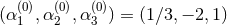 , which is not the Gauss–Bonnet invariant. Notice also that this model is not
usually studied in modified quadratic gravity theory, as one usually concentrates on the terms that have an
explicit scalar field coupling.
, which is not the Gauss–Bonnet invariant. Notice also that this model is not
usually studied in modified quadratic gravity theory, as one usually concentrates on the terms that have an
explicit scalar field coupling.
The field equations of this theory can be read directly from Eq. (27), but we repeat them here for completeness:

One could in principle rewrite this in terms of the Riemann and Ricci tensors, but the expressions become quite complicated, as calculated explicitly in Eqs. (2) and (3) of [473*]. Due to the absence of a dynamical degree of freedom coupling to the modifications to the Einstein–Hilbert action, this theory is not covariantly conserved in vacuum. By this we mean that the covariant divergence of Eq. (41) does not vanish in vacuum, thus violating the weak-equivalence principle and leading to additional equations that might over-constrain the system. In the presence of matter, the equations of motion will not be given by the vanishing of the covariant divergence of the matter stress-energy alone, but now there will be additional geometric terms.
Given these field equations, one can linearize them about a flat background to find the evolution equations for the metric perturbation [326*, 325*]
where the term proportional to
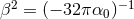 acts like a mass term. Here, one has imposed the
transverse-traceless gauge (a refinement of Lorenz gauge), which can be shown to exist [326*, 325*]. Clearly,
even though the full non-linear equations are not covariantly conserved, its linearized version is, as one can
easily show that the divergence of the left-hand side of Eq. (42*) vanishes. Because of these
features, if one works perturbatively in
acts like a mass term. Here, one has imposed the
transverse-traceless gauge (a refinement of Lorenz gauge), which can be shown to exist [326*, 325*]. Clearly,
even though the full non-linear equations are not covariantly conserved, its linearized version is, as one can
easily show that the divergence of the left-hand side of Eq. (42*) vanishes. Because of these
features, if one works perturbatively in  , then such a theory will only possess the two usual
transverse-traceless (spin-2) polarization modes, i.e., it is perturbatively of type
, then such a theory will only possess the two usual
transverse-traceless (spin-2) polarization modes, i.e., it is perturbatively of type  in the
  classification [161].
Let us now discuss whether such a theory satisfies the properties discussed in Section 2.1.
Non-commutative geometry theories clearly possess the fundamental property, as one can always take
 (or equivalently
  ) to recover GR. Therefore, there must exist a sufficiently small
  such that all precision tests carried out to date are satisfied. As for the existence and stability of known
solutions, [326*, 325*] have shown that Minkowski spacetime is stable only for
such that all precision tests carried out to date are satisfied. As for the existence and stability of known
solutions, [326*, 325*] have shown that Minkowski spacetime is stable only for  , as otherwise a
tachyonic term appears in the evolution of the metric perturbation, as can be seen from Eq. (42*). This then
automatically implies that
, as otherwise a
tachyonic term appears in the evolution of the metric perturbation, as can be seen from Eq. (42*). This then
automatically implies that  must be real.
Current constraints on Weyl terms of this form come mostly from solar system experiments.
Ni [328*] recently studied an action of the form of Eq. (38) minimally coupled to matter in light of
solar system experiments. He calculated the relativistic Shapiro time-delay and light deflection
about a massive body in this theory and found that observations of the Cassini satellite place
constraints on 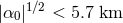 [328]. This is currently the strongest bound we are aware of on
 .
.
Many solutions of GR are preserved in non-commutative geometries. Regarding black holes, all solutions that are Ricci flat (vacuum solutions of the Einstein equations) are also solutions to Eq. (41). This is because by the second Bianchi identity, one can show that
and the right-hand side vanishes in vacuum, forcing the entire left-hand side of Eq. (41) to vanish. However, this is not so for neutron stars where the equations of motion are likely to be modified, unless they are static [324]. Moreover, as of now there has been no stability analysis of black-hole or stellar solutions and no study of whether the theory is well posed as an initial-value problem, even as an effective theory. Thus, except for the fundamental property, it is not clear that non-commutative geometries satisfy any of the other criteria listed in Section 2.1.
2.3.6 Gravitational parity violation
Parity, the symmetry transformation that flips the sign of the spatial triad, has been found to be broken in the standard model of elementary interactions. Only the combination of charge conjugation, parity transformation and time inversion (CPT) still remains a true symmetry of the standard model. Experimentally, it is curious that the weak interaction exhibits maximal parity violation, while other fundamental forces seem to not exhibit any. Theoretically, parity violation unavoidably arises in the standard model [55, 8, 21], as there exist one-loop chiral anomalies that give rise to parity-violating terms coupled to lepton number [428]. In certain sectors of string theory, such as in heterotic and Type I superstring theories, parity violation terms are also generated through the Green–Schwarz gauge anomaly-canceling mechanism [204, 355, 12]. Finally, in loop quantum gravity [41], the scalarization of the Barbero–Immirzi parameter coupled to fermions leads to an effective action that contains parity-violating terms [406, 90, 311, 192]. Even without a particular theoretical model, one can show that effective field theories of inflation generically contain non-vanishing, second-order, parity-violating curvature corrections to the Einstein–Hilbert action [429]. Alternatively, phenomenological parity-violating extensions of GR have been proposed through a scalarization of the fundamental constants of nature [115].
One is then naturally led to ask whether the gravitational interaction is parity invariant in the strong
field. A violation of parity invariance would occur if the Einstein–Hilbert action were modified through a
term that involved a Levi-Civita tensor and parity invariant tensors or scalars. Let us try to
construct such terms with only single powers of the Riemann tensor and a single scalar field
 :
:
Option (ia) and (ib) vanish by the Bianchi identities. Options (ic) and (id) include the commutator of covariant derivatives, which can be rewritten in terms of a Riemann tensor, and thus it leads to terms that are at least quadratic in the Riemann tensor. Therefore, no scalar can be constructed that includes contractions with the Levi-Civita tensor from a single Riemann curvature tensor and a single field. One can try to construct a scalar from the Ricci tensor

but again (iia) vanishes by the symmetries of the Ricci tensor, while (iib) involves the commutator of covariant derivatives, which introduces another power of the curvature tensor. Obviously, the only term one can write with the Ricci scalar would lead to a double commutator of covariant derivatives, leading to extra factors of the curvature tensor.
One is then forced to consider either theories with two mutually-independent fields or theories with
quadratic curvature tensors. Of the latter, the only combination that can be constructed and that does not
vanish by the Bianchi identities is the Pontryagin density, i.e.,  , and therefore, the action [245*, 17*]

 prefactor to follow historical conventions. This action defines non-dynamical Chern–Simons
modified gravity, initially proposed by Jackiw and Pi [245*, 17*]. Notice that this is the same as the term
proportional to
prefactor to follow historical conventions. This action defines non-dynamical Chern–Simons
modified gravity, initially proposed by Jackiw and Pi [245*, 17*]. Notice that this is the same as the term
proportional to  in the quadratic gravity action of Eq. (26), except that here
  is prior geometry, i.e.,
it does not possess self-consistent dynamics or an evolution equation. Such a term violates parity
invariance because the Pontryagin density is a pseudo-scalar, while
is prior geometry, i.e.,
it does not possess self-consistent dynamics or an evolution equation. Such a term violates parity
invariance because the Pontryagin density is a pseudo-scalar, while  is assumed to be a
scalar.
is assumed to be a
scalar.
The field equations for this theory are7
which is simply Eq. (27) with
 set to zero and no stress-energy for
  . Clearly, these field
equations are not covariantly conserved in vacuum, i.e., taking the covariant divergence one finds the
constraint
This constraint restricts the space of allowed solutions, for example disallowing the Kerr metric [207*].
Therefore, it might seem that the evolution equations for the metric are now overconstrained, given that the
field equations provide 10 differential conditions for the 10 independent components of the metric tensor,
while the constraint adds one additional, independent differential condition. Moreover, unless the
Pontryagin constraint, Eq. (47*), is satisfied, matter fields will not evolve according to
. Clearly, these field
equations are not covariantly conserved in vacuum, i.e., taking the covariant divergence one finds the
constraint
This constraint restricts the space of allowed solutions, for example disallowing the Kerr metric [207*].
Therefore, it might seem that the evolution equations for the metric are now overconstrained, given that the
field equations provide 10 differential conditions for the 10 independent components of the metric tensor,
while the constraint adds one additional, independent differential condition. Moreover, unless the
Pontryagin constraint, Eq. (47*), is satisfied, matter fields will not evolve according to 
 , thus
violating the equivalence principle.
, thus
violating the equivalence principle.
From the field equations, we can derive an evolution equation for the metric perturbation when linearizing about a flat background, namely
in a transverse-traceless gauge, which can be shown to exist in this theory [11*, 460*]. The constraint of Eq. (47*) is identically satisfied to second order in the metric perturbation. However, without further information about
 one cannot proceed any further, except for a few general observations. As is clear
from Eq. (48*), the evolution equation for the metric perturbation can contain third time derivatives, which
generically will lead to instabilities. In fact, as shown in [13] the general solution to these equations will
contain exponentially growing and decaying modes. However, the theory defined by Eq. (45*) is an effective
theory, and thus, there can be higher-order operators not included in this action that may stabilize the
solution. Regardless, when studying this theory order-reduction is necessary if one is to consider it an
effective model.
one cannot proceed any further, except for a few general observations. As is clear
from Eq. (48*), the evolution equation for the metric perturbation can contain third time derivatives, which
generically will lead to instabilities. In fact, as shown in [13] the general solution to these equations will
contain exponentially growing and decaying modes. However, the theory defined by Eq. (45*) is an effective
theory, and thus, there can be higher-order operators not included in this action that may stabilize the
solution. Regardless, when studying this theory order-reduction is necessary if one is to consider it an
effective model.
Let us now discuss the properties of such an effective theory. Because of the structure of the
modification to the field equations, one can always choose a sufficiently small value for  such that all
solar system tests are satisfied. In fact, one can see from the equations in this section that in the limit
such that all
solar system tests are satisfied. In fact, one can see from the equations in this section that in the limit
 , one recovers GR. Non-dynamical Chern–Simons gravity leads to modifications to the
non-radiative (near-zone) metric in the gravitomagnetic sector, leading to corrections to Lense–Thirring
precession [14, 15]. This fact has been used to constrain the theory through observations of the orbital
motion of the LAGEOS satellites [388*] to
, one recovers GR. Non-dynamical Chern–Simons gravity leads to modifications to the
non-radiative (near-zone) metric in the gravitomagnetic sector, leading to corrections to Lense–Thirring
precession [14, 15]. This fact has been used to constrain the theory through observations of the orbital
motion of the LAGEOS satellites [388*] to  , or equivalently
  .
However, much better constraints can be placed through observations of the binary pulsar [472, 18]:
.
However, much better constraints can be placed through observations of the binary pulsar [472, 18]:
 .
.
Some of the sub-properties of the fundamental requirement are satisfied in non-dynamical Chern–Simons
gravity. On the one hand, all spherically-symmetric metrics that are solutions to the Einstein equations
are also solutions in this theory for a “canonical” scalar field ( ) [207]. On the other
hand, axisymmetric solutions to the Einstein equations are generically not solutions in this
theory. Moreover, although spherically-symmetric solutions are preserved, perturbations of such
spacetimes that are solutions to the Einstein equations are not generically solutions to the
modified theory [470*]. What is perhaps worse, the evolution of perturbations to non-spinning black
holes have been found to be generically overconstrained [470]. This is a consequence of the lack
of scalar field dynamics in the modified theory, which, via Eq. (47*), tends to overconstrain
it. Such a conclusion also suggests that this theory does not posses a well-posed initial-value
problem.
) [207]. On the other
hand, axisymmetric solutions to the Einstein equations are generically not solutions in this
theory. Moreover, although spherically-symmetric solutions are preserved, perturbations of such
spacetimes that are solutions to the Einstein equations are not generically solutions to the
modified theory [470*]. What is perhaps worse, the evolution of perturbations to non-spinning black
holes have been found to be generically overconstrained [470]. This is a consequence of the lack
of scalar field dynamics in the modified theory, which, via Eq. (47*), tends to overconstrain
it. Such a conclusion also suggests that this theory does not posses a well-posed initial-value
problem.
One can argue that non-dynamical Chern–Simons gravity is well-motivated from fundamental theories [17*], except that in the latter, the scalar field is always dynamical, instead of having to be prescribed a priori. Thus, perhaps the strongest motivation for such a model is as a phenomenological proxy to test whether the gravitational interaction remains parity invariant in the strong field, a test that is uniquely suited to this modified model.
2.4 Currently unexplored theories in the gravitational-wave sector
The list of theories we have described here is by no means exhaustive. In fact, there are many fascinating theories that we have chosen to leave out because they have not yet been analyzed in the gravitational wave context in detail. Examples of these include the following:
- Einstein-Aether Theory [247] and Hořava–Lifshitz Theory [234];
- Standard Model Extension [109];
- Eddington-inspired Born–Infeld gravity [48];
- New Massive Gravity [60, 136] and Bi-Gravity Theories [349, 346, 219, 220].
We will update this review with a description of these theories, once a detailed gravitational-wave study for compact binaries or supernovae sources is carried out and the predictions for the gravitational waveform observables are made for any physical system plausibly detectable by current or near future gravitational-wave experiments.
 |
 |
 |
Living Rev. Relativity, 16 (2013), 9, doi:10.12942/lrr-2013-9, URL (accessed <date>): http://www.livingreviews.org/lrr-2013-9.
 This work is licensed under a Creative Commons License.
© The author(s), except where otherwise noted.
This work is licensed under a Creative Commons License.
© The author(s), except where otherwise noted.