4 Testing Techniques
4.1 Coalescence analysis
Gravitational waves emitted during the inspiral, merger and ringdown of compact binaries are the most studied in the context of data analysis and parameter estimation. In this section, we will review some of the main data analysis techniques employed in the context of parameter estimation and tests of GR. We begin with a discussion of matched filtering and Fisher theory (for a detailed review, see [173, 103, 125*, 174*, 248]). We then continue with a discussion of Bayesian parameter estimation and hypothesis testing (for a detailed review, see [387, 205, 123, 294*]).
4.1.1 Matched filtering and Fisher’s analysis
When the detector noise  is Gaussian and stationary, and when the signal
  is known very well,
the optimal detection strategy is matched filtering. For any given realization, such noise can be
characterized by its power spectral density
is known very well,
the optimal detection strategy is matched filtering. For any given realization, such noise can be
characterized by its power spectral density  , defined via

The detectability of a signal is determined by its signal-to-noise ratio or SNR, which is defined via
where
 is a template with parameters
  and we have defined the inner product
If the templates do not exactly match the signal, then the SNR is reduced by a factor of
and we have defined the inner product
If the templates do not exactly match the signal, then the SNR is reduced by a factor of 
 , called the
match:
where
, called the
match:
where 
 is the mismatch.
For the noise assumptions made here, the probability of measuring  in the detector output, given a
template
in the detector output, given a
template  , is given by

 that best fits the signal is that with best-fit parameters such that the argument
of the exponential is minimized. For large SNR, the best-fit parameters will have a multivariate Gaussian
distribution centered on the true values of the signal
that best fits the signal is that with best-fit parameters such that the argument
of the exponential is minimized. For large SNR, the best-fit parameters will have a multivariate Gaussian
distribution centered on the true values of the signal  , and thus, the waveform parameters that best fit
the signal minimize the argument of the exponential. The parameter errors
, and thus, the waveform parameters that best fit
the signal minimize the argument of the exponential. The parameter errors  will be distributed
according to
where
will be distributed
according to
where 
 is the Fisher matrix
The root-mean-squared (
is the Fisher matrix
The root-mean-squared (
 ) error on a given parameter
  is then
where
is then
where 
 is the variance-covariance matrix and summation is not implied in Eq. (83*) (
 denotes a particular element of the vector
  ). This root-mean-squared error is sometimes referred to as
the statistical error in the measurement of
). This root-mean-squared error is sometimes referred to as
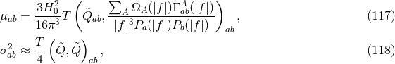
the statistical error in the measurement of  . One can use Eq. (83*) to estimate how well modified gravity
parameters can be measured. Put another way, if a gravitational wave were detected and found consistent
with GR, Eq. (83*) would provide an estimate of how close to zero these modified gravity parameters would
have to be.
. One can use Eq. (83*) to estimate how well modified gravity
parameters can be measured. Put another way, if a gravitational wave were detected and found consistent
with GR, Eq. (83*) would provide an estimate of how close to zero these modified gravity parameters would
have to be.
The Fisher method to estimate projected constraints on modified gravity theory parameters is as
follows. First, one constructs a waveform model in the particular modified gravity theory one wishes to
constrain. Usually, this waveform will be similar to the GR one, but it will contain an additional parameter,
 , such that the template parameters are now
  plus
plus  . Let us assume that as
  , the modified
gravity waveform reduces to the GR expectation. Then, the accuracy to which
, the modified
gravity waveform reduces to the GR expectation. Then, the accuracy to which  can be measured, or
the accuracy to which we can say
can be measured, or
the accuracy to which we can say  is zero, is approximately
  , where the Fisher
matrix associated with this variance-covariance matrix must be computed with the non-GR
model evaluated at the GR limit (
, where the Fisher
matrix associated with this variance-covariance matrix must be computed with the non-GR
model evaluated at the GR limit ( ). Such a method for estimating how well modified
gravity theories can be constrained was pioneered by Will in [436*, 353], and since then, it has
been widely employed as a first-cut estimate of the accuracy to which different theories can be
constrained.
). Such a method for estimating how well modified
gravity theories can be constrained was pioneered by Will in [436*, 353], and since then, it has
been widely employed as a first-cut estimate of the accuracy to which different theories can be
constrained.
The Fisher method described above can dangerously lead to incorrect results if abused [414, 415]. One
must understand that this method is suitable only if the noise is stationary and Gaussian and if the SNR is
sufficiently large. How large an SNR is required for Fisher methods to work depends somewhat on the
signals considered, but usually for applications concerning tests of GR, one would be safe with  or
so. In real data analysis, the first two conditions are almost never satisfied. Moreover, the first
detections that will be made will probably be of low SNR, i.e.,
or
so. In real data analysis, the first two conditions are almost never satisfied. Moreover, the first
detections that will be made will probably be of low SNR, i.e.,  , for which again the
Fisher method fails. In such cases, more sophisticated parameter estimation methods need to be
employed.
, for which again the
Fisher method fails. In such cases, more sophisticated parameter estimation methods need to be
employed.
4.1.2 Bayesian theory and model testing
Bayesian theory is ideal for parameter estimation and model selection. Let us then assume that a detection
has been made and that the gravitational wave signal in the data can be described by some model  ,
parameterized by the vector
,
parameterized by the vector  . Using Bayes’ theorem, the posterior distribution function (PDF) or
the probability density function for the model parameters, given data
. Using Bayes’ theorem, the posterior distribution function (PDF) or
the probability density function for the model parameters, given data  and model
  , is
, is

 represents our prior beliefs of the parameter
range in model
represents our prior beliefs of the parameter
range in model  . The marginalized likelihood or evidence, is the normalization constant
which clearly guarantees that the integral of Eq. (84*) integrates to unity. The quantity
. The marginalized likelihood or evidence, is the normalization constant
which clearly guarantees that the integral of Eq. (84*) integrates to unity. The quantity 
 is the
likelihood function, which is simply given by Eq. (80*), with a given normalization. In that equation we used
slightly different notation, with
is the
likelihood function, which is simply given by Eq. (80*), with a given normalization. In that equation we used
slightly different notation, with  being the data
  and
and  the template associated with model
  and parameterized by
  . The marginalized PDF, which represents the probability density function for a
given parameter
. The marginalized PDF, which represents the probability density function for a
given parameter  (recall that
  is a particular element of
  ), after marginalizing over all other
parameters, is given by
where the integration is not to be carried out over
), after marginalizing over all other
parameters, is given by
where the integration is not to be carried out over 
 .
.
Let us now switch gears to model selection. In hypothesis testing, one wishes to determine whether the
data is more consistent with hypothesis A (e.g., that a GR waveform correctly models the signal) or with
hypothesis B (e.g., that a non-GR waveform correctly models the signal). Using Bayes’ theorem, the PDF
for model  given the data is

 is the prior probability of hypothesis
  , namely the strength of our prior belief that
hypothesis
, namely the strength of our prior belief that
hypothesis  is correct. The normalization constant
  is given by
where the integral is to be taken over all models. Thus, it is clear that this normalization constant does
not depend on the model. Similar relations hold for hypothesis
is given by
where the integral is to be taken over all models. Thus, it is clear that this normalization constant does
not depend on the model. Similar relations hold for hypothesis 
 by replacing
  in
Eq. (87*).
in
Eq. (87*).
When hypothesis A and B refer to fundamental theories of nature we can take different viewpoints
regarding the priors. If we argue that we know nothing about whether hypothesis A or B better describes
nature, then we would assign equal priors to both hypotheses. If, on the other hand, we believe GR is the
correct theory of nature, based on all previous experiments performed in the solar system and with binary
pulsars, then we would assign  . This assigning of priors necessarily biases the inferences
derived from the calculated posteriors, which is sometimes heavily debated when comparing Bayesian theory
to a frequentist approach. However, this “biasing” is really unavoidable and merely a reflection of
our state of knowledge of nature (for a more detailed discussion on such issues, please refer
to [294]).
. This assigning of priors necessarily biases the inferences
derived from the calculated posteriors, which is sometimes heavily debated when comparing Bayesian theory
to a frequentist approach. However, this “biasing” is really unavoidable and merely a reflection of
our state of knowledge of nature (for a more detailed discussion on such issues, please refer
to [294]).
The integral over all models in Eq. (88*) can never be calculated in practice, simply because
we do not know all models. Thus, one is forced to investigate relative probabilities between
models, such that the normalization constant  cancels out. The odds ratio is defined by

 is the Bayes factor and the prefactor
  is the prior odds. The
odds-ratio is a convenient quantity to calculate because the evidence
is the prior odds. The
odds-ratio is a convenient quantity to calculate because the evidence  , which is difficult to compute,
actually cancels out. Recently, Vallisneri [416] has investigated the possibility of calculating the odds-ratio
using only frequentist tools and without having to compute full evidences. The odds-ratio should
be interpreted as the betting-odds of model
, which is difficult to compute,
actually cancels out. Recently, Vallisneri [416] has investigated the possibility of calculating the odds-ratio
using only frequentist tools and without having to compute full evidences. The odds-ratio should
be interpreted as the betting-odds of model  over model
  . For example, an odds-ratio
of unity means that both models are equally supported by the data, while an odds-ratio of
. For example, an odds-ratio
of unity means that both models are equally supported by the data, while an odds-ratio of
 means that there is a 100 to 1 odds that model
  better describes the data than model
 .
.
The main difficulty in Bayesian inference (both in parameter estimation and model selection) is sampling the PDF sufficiently accurately. Several methods have been developed for this purpose, but currently the two main workhorses in gravitational-wave data analysis are Markov Chain Monte Carlo and Nested Sampling. In the former, one samples the likelihood through the Metropolis–Hastings algorithm [314, 221, 122, 367]. This is computationally expensive in high-dimensional cases, and thus, there are several techniques to improve the efficiency of the method, e.g., parallel tempering [402]. Once the PDF has been sampled, one can then calculate the evidence integral, for example via thermodynamic integration [420, 167, 419]. In Nested Sampling, the evidence is calculated directly by laying out a fixed number of points in the prior volume, which are then allowed to move and coalesce toward regions of high posterior probability. With the evidence in hand, one can then infer the PDF. As in the previous case, Nested Sampling can be computationally expensive in high-dimensional cases.
Del Pozzo et al. [142*] were the first to carry out a Bayesian implementation of model selection in the context of tests of GR. Their analysis focused on tests of a particular massive graviton theory, using the gravitational wave signal from quasi-circular inspiral of non-spinning black holes. Cornish et al. [124*, 376*] extended this analysis by considering model-independent deviations from GR, using the parameterized post-Einsteinian (ppE) approach (Section 5.3.4) [467*]. Recently, this was continued by Li et al. [290*, 291], who carried out a similar analysis on a large statistical sample of Advanced LIGO (aLIGO) detections using simulated data and a restricted ppE model. All of these studies suggest that Bayesian tests of GR are possible, given sufficiently-high SNR events. Of course, whether deviations from GR are observable will depend on the strong-field character and strength of the deviation, as well as the availability of sufficiently-accurate GR waveforms.
4.1.3 Systematics in model selection
The model selection techniques described above are affected by other systematics present in data analysis. In general, we can classify these into the following [417*]:
- Mismodeling Systematic, caused by inaccurate models of the gravitational-wave template.
- Instrumental Systematic, caused by inaccurate models of the gravitational-wave response.
- Astrophysical Systematic, caused by inaccurate models of the astrophysical environment.
Mismodeling systematics are introduced due to the lack of an exact solution to the Einstein equations from which to extract an exact template, given a particular astrophysical scenario. Inspiral templates, for example, are approximated through post-Newtonian theory and become increasingly less accurate as the binary components approach each other. Cutler and Vallisneri [127] were the first to carry out a formal and practical investigation of such a systematic in the context of parameter estimation from a frequentist approach.
Mismodeling systematics will prevent us from testing GR effectively with signals that we do not understand sufficiently well. For example, when considering signals from black hole coalescences, if the the total mass of the binary is sufficiently high, the binary will merge in band. The higher the total mass, the fewer the inspiral cycles that will be in band, until eventually only the merger is in band. Since the merger phase is the least understood phase, it stands to reason that our ability to test GR will deteriorate as the total mass increases. Of course, we do understand the ringdown phase very well, and tests of the no-hair theorem would be allowed during this phase, provided a sufficiently-high SNR [65*]. On the other hand, for neutron star binaries or very–low-mass black-hole binaries, the merger phase is expected to be essentially out of band for aLIGO (above 1 kHz), and thus, the noise spectrum itself may shield us from our ignorance.
Instrumental systematics are introduced by our ignorance of the transfer function, which connects the detector output to the incoming gravitational waves. Through sophisticated calibration studies with real data, one can approximate the transfer function very well [4*, 1]. However, this function is not time-independent, because the noise in the instrument is not stationary or Gaussian. Thus, un-modeled drifts in the transfer function can introduce systematics in parameter estimation that are as large as 10% in the amplitude and the phase [4].
Instrumental systematics can affect tests of GR, if these are performed with a single instrument. However, one expects multiple detectors to be online in the future and for gravitational-wave detections to be made in several of them simultaneously. Instrumental systematics should be present in all such detections, but since the noise will be mostly uncorrelated between different instruments, one should be able to ameliorate its effects through cross-correlating outputs from several instruments.
Astrophysical systematics are induced by our lack of a priori knowledge of the gravitational wave source. As explained above, matched filtering requires knowledge of a waveform template with which to filter the data. Usually, we assume the sources are in a perfect vacuum and isolated. For example, when considering inspiral signals, we ignore any third bodies, electric or magnetic fields, neutron star hydrodynamics, the expansion of the universe, etc. Fortunately, however, most of these effects are expected to be small: the probability of finding third bodies sufficiently close to a binary system is very small [463*]; for low redshift events, the expansion of the universe induces an acceleration of the center of mass, which is also very small [468*]; electromagnetic fields and neutron-star hydrodynamic effects may affect the inspiral of black holes and neutron stars, but not until the very last stages, when most signals will be out of band anyways. For example, tidal deformation effects enter a neutron-star–binary inspiral waveform at 5 post-Newtonian order, which therefore affects the signal outside of the most sensitive part of the aLIGO sensitivity bucket.
Perhaps the most dangerous source of astrophysical systematics is due to the assumptions made about the astrophysical systems we expect to observe. For example, when considering neutron-star–binary inspirals, one usually assumes the orbit will have circularized by the time it enters the sensitivity band. Moreover, one assumes that any residual spin angular momentum that the neutron stars may possess is very small and aligned or counter-aligned with the orbital angular momentum. These assumptions certainly simplify the construction of waveform templates, but if they happen to be wrong, they would introduce mismodeling systematics that could also affect parameter estimation and tests of GR.
4.2 Burst analyses
In alternative theories of gravity, gravitational-wave sources such as core collapse supernovae may result in the production of gravitational waves in more than just the plus and cross-polarizations [384, 380, 216, 334, 333, 369]. Indeed, the near-spherical geometry of the collapse can be a source of scalar breathing-mode gravitational waves. However, the precise form of the waveform is unknown because it is sensitive to the initial conditions.
When searching for un-modeled bursts in alternative theories of gravity, a general approach involves
optimized linear combinations of data streams from all available detectors to form maximum likelihood
estimates of the waveforms in the various polarizations, and the use of null streams. In the context of
ground-based detectors and GR, these ideas were first explored by Gürsel and Tinto [212*] and later by
Chatterji et al. [101*] with the aim of separating false-alarm events from real detections. The main idea was
to construct a linear combination of data streams received by a network of detectors, so that the
combination contained only noise. Of course, in GR one need only include  and
and  polarizations, and
thus a network of three detectors suffices. This concept can be extended to develop null tests of GR, as
originally proposed by Chatziioannou et al. [102*] and recently implemented by Hayama et
al. [228*].
polarizations, and
thus a network of three detectors suffices. This concept can be extended to develop null tests of GR, as
originally proposed by Chatziioannou et al. [102*] and recently implemented by Hayama et
al. [228*].
Let us consider a network of  detectors with uncorrelated noise and a detection by all
  detectors. For a source that emits gravitational waves in the direction
  , a single data point (either in the
time-domain, or a time-frequency pixel) from an array of
, a single data point (either in the
time-domain, or a time-frequency pixel) from an array of  detectors (either pulsars or interferometers)
can be written as
detectors (either pulsars or interferometers)
can be written as

 is a vector with the noise. The antenna pattern functions are given by the matrix,
For simplicity we have suppressed the sky-location dependence of the antenna pattern functions. These can
either be the interferometric antenna pattern functions in Eqs. (58*), or the pulsar response functions in
Eqs. (69*). For interferometers, since the breathing and longitudinal antenna pattern response functions are
degenerate, and even though
is a vector with the noise. The antenna pattern functions are given by the matrix,
For simplicity we have suppressed the sky-location dependence of the antenna pattern functions. These can
either be the interferometric antenna pattern functions in Eqs. (58*), or the pulsar response functions in
Eqs. (69*). For interferometers, since the breathing and longitudinal antenna pattern response functions are
degenerate, and even though ![⌊ ⌋ F +F × F x F y Fb F ℓ | 1+ 1× 1x 1y 1b 1ℓ| [ F + F × F x F y F b F ℓ] ≡ || F2. F 2. F.2 F2. F.2 F.2|| . (92 ) ⌈ .. .. .. .. .. .. ⌉ F +F × F x F yF b F ℓ D D D D D D](article561x.gif)
 is a
is a  matrix, there are only five linearly-independent
vectors [81, 80, 102*, 228*].
matrix, there are only five linearly-independent
vectors [81, 80, 102*, 228*].
If we do not know the form of the signal present in our data, we can obtain maximum likelihood
estimators for it. For simplicity, let us assume the data are Gaussian and of unit variance (the latter can be
achieved by whitening the data). Just as we did in Eq. (80*), we can write the probability of obtaining
datum  , in the presence of a gravitational wave
  as
as
![1 [ 1 ] P(d |h ) = ----D∕2-exp − -|d − F h |2 . (93 ) (2π) 2](article566x.gif)
![[ ] L ≡ ln P-(d-|h)-= 1- |d|2 − |d − F h |2 . (94 ) P (d|0) 2](article567x.gif)


 is a projection operator that projects the data into the subspace spanned by
  . An
orthogonal projector can also be constructed,
which projects the data onto a sub-space orthogonal to
. An
orthogonal projector can also be constructed,
which projects the data onto a sub-space orthogonal to 
 . Thus one can construct a certain linear
combination of data streams that has no component of a certain polarization by projecting them to a
direction orthogonal to the direction defined by the beam pattern functions of this polarization mode
This is called a null stream and, in the context of GR, it was introduced as a means of separating
false-alarm events due, say, to instrumental glitches from real detections [212*, 101*].
. Thus one can construct a certain linear
combination of data streams that has no component of a certain polarization by projecting them to a
direction orthogonal to the direction defined by the beam pattern functions of this polarization mode
This is called a null stream and, in the context of GR, it was introduced as a means of separating
false-alarm events due, say, to instrumental glitches from real detections [212*, 101*].

With just three independent detectors, we can choose to eliminate the two tensor modes (the plus and cross-polarizations) and construct a GR null stream: a linear combination of data streams that contains no signal consistent within GR, but could contain a signal in another gravitational theory, as illustrated in Figure 4*. With such a GR null stream, one can carry out null tests of GR and study whether such a stream contains any statistically-significant deviations from noise. Notice that this approach does not require a template; if one were parametrically constructed, such as in [102*], more powerful null tests could be applied. In the future, we expect several gravitational wave detectors to be online: the two aLIGO ones in the United States, Advanced VIRGO (adVirgo) in Italy, LIGO-India in India, and KAGRA in Japan. Given a gravitational-wave observation that is detected by all five detectors, one can then construct three GR null streams, each with power in a signal direction.
For pulsar timing experiments where one is dealing with data streams of about a few tens of pulsars, waveform reconstruction for all polarization states, as well as numerous null streams, can be constructed.
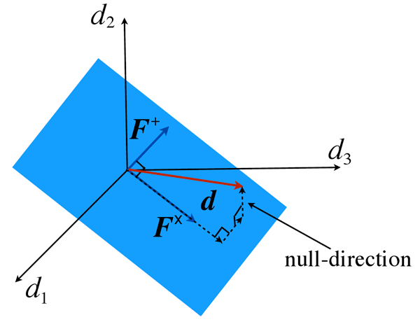
 orthogonal to the GR subspace
spanned by
orthogonal to the GR subspace
spanned by  and
and  , along with a perpendicular subspace, for 3 detectors to build the GR
null stream.
, along with a perpendicular subspace, for 3 detectors to build the GR
null stream.4.3 Stochastic background searches
Much work has been done on the response of ground-based interferometers to non-tensorial polarization modes, stochastic background detection prospects, and data analysis techniques [299, 323, 191, 329*, 121]. In the context of pulsar timing, the first work to deal with the detection of such backgrounds in the context of alternative theories of gravity is due to Lee et al. [284*], who used a coherence statistic approach to the detection of non-Einsteinian polarizations. They studied the number of pulsars required to detect the various extra polarization modes, and found that pulsar timing arrays are especially sensitive to the longitudinal mode. Alves and Tinto [22*] also found enhanced sensitivity to longitudinal and vector modes. Here we follow the work in [329*, 99*] that deals with the LIGO and pulsar timing cases using the optimal statistic, a cross-correlation that maximizes the SNR.
In the context of the optimal statistic, the derivations of the effect of extra polarization states for ground-based instruments and pulsar timing are very similar. We begin with the metric perturbation written in terms of a plane wave expansion, as in Eq. (50*). If we assume that the background is unpolarized, isotropic, and stationary, we have that
where
 is the gravitational-wave power spectrum for polarization
  .
.  is related to the
energy density in gravitational waves per logarithmic frequency interval for that polarization through
where
is related to the
energy density in gravitational waves per logarithmic frequency interval for that polarization through
where 
 is the closure density of the universe, and
is the energy density in gravitational waves for polarization
is the closure density of the universe, and
is the energy density in gravitational waves for polarization 
 . It follows from the plane wave expansion
in Eq. (51*), along with Eqs. (101*) and (102*) in Eq. (103*), that
and therefore
. It follows from the plane wave expansion
in Eq. (51*), along with Eqs. (101*) and (102*) in Eq. (103*), that
and therefore


For both ground-based interferometers and pulsar-timing experiments, an isotropic stochastic
background of gravitational waves appears in the data as correlated noise between measurements from
different instruments. The data set from the  instrument is of the form

 corresponds to the gravitational-wave signal and
  to noise. The noise is
assumed in this case to be stationary and Gaussian, and uncorrelated between different detectors,
for
to noise. The noise is
assumed in this case to be stationary and Gaussian, and uncorrelated between different detectors,
for 
 .
.
Since the gravitational-wave signal is correlated, we can use cross-correlations to search for it. The cross-correlation statistic is defined as
where
 is a filter function to be determined. Henceforth, no summation is implied on the
detector indices
is a filter function to be determined. Henceforth, no summation is implied on the
detector indices  . At this stage it is not clear why
  depends on the pair of data sets
being correlated. We will show how this comes about later. The optimal filter is determined by maximizing
the expected SNR
Here
depends on the pair of data sets
being correlated. We will show how this comes about later. The optimal filter is determined by maximizing
the expected SNR
Here 
 is the mean
  and
and  is the square root of the variance
  .
.
The expressions for the mean and variance of the cross-correlation statistic,  and
and  respectively,
take the same form for both pulsar timing and ground-based instruments. In the frequency domain,
Eq. (109*) becomes
respectively,
take the same form for both pulsar timing and ground-based instruments. In the frequency domain,
Eq. (109*) becomes

 is then
where
is then
where 
 is the finite time approximation to the delta function,
  . With this in
hand, the mean of the cross-correlation statistic is
and the variance in the weak signal limit is
where the one-sided power spectra of the noise are defined by
in analogy to Eq. (76*), where
. With this in
hand, the mean of the cross-correlation statistic is
and the variance in the weak signal limit is
where the one-sided power spectra of the noise are defined by
in analogy to Eq. (76*), where 
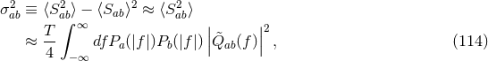

 plays here the role of
  .
.
The mean and variance can be rewritten more compactly if we define a positive-definite inner product using the noise power spectra of the two data streams
again in analogy to the inner product in Eq. (78*), when considering inspirals. Using this definition where we recall that the capital Latin indices
 stand for the polarization content. From the
definition of the SNR and the Schwartz’s inequality, it follows that the optimal filter is given by
where
stand for the polarization content. From the
definition of the SNR and the Schwartz’s inequality, it follows that the optimal filter is given by
where 
 is an arbitrary normalization constant, normally chosen so that the mean of the statistic gives
the amplitude of the stochastic background.
is an arbitrary normalization constant, normally chosen so that the mean of the statistic gives
the amplitude of the stochastic background.
The differences in the optimal filter between interferometers and pulsars arise only from
differences in the overlap reduction functions,  . For ground-based instruments, the signal
data
. For ground-based instruments, the signal
data  are the strains given by Eq. (57*). The overlap reduction functions are then given by

 and
and  are the locations of the two interferometers. The integrals in this case all have
solutions in terms of spherical Bessel functions [329*], which we do not summarize here for
brevity.
are the locations of the two interferometers. The integrals in this case all have
solutions in terms of spherical Bessel functions [329*], which we do not summarize here for
brevity.
For pulsar timing arrays, the signal data  are the redshifts
  , given by Eq. (63*). The overlap
reduction functions are then given by
, given by Eq. (63*). The overlap
reduction functions are then given by

 and
and  are the distances to the two pulsars. For all transverse modes pulsar timing
experiments are in a regime where the exponential factors in Eq. (121*) can be neglected [30, 99*], and the
overlap reduction functions effectively become frequency independent. For the
are the distances to the two pulsars. For all transverse modes pulsar timing
experiments are in a regime where the exponential factors in Eq. (121*) can be neglected [30, 99*], and the
overlap reduction functions effectively become frequency independent. For the  and
and  mode the
overlap reduction function becomes
where
mode the
overlap reduction function becomes
where ![{ [ ( ) ]} + 1 1 − cosξab 1 − cosξab 1 Γab = 3 --+ ---------- ln ---------- − -- , (122 ) 3 2 2 6](article635x.gif)
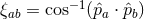 is the angle between the two pulsars. This quantity is proportional to the
Hellings and Downs curve [231]. For the breathing mode, the overlap reduction function takes the closed
form expression [284*]:
For the vector and longitudinal modes the overlap reduction functions remain frequency dependent and
there are no general analytic solutions.
is the angle between the two pulsars. This quantity is proportional to the
Hellings and Downs curve [231]. For the breathing mode, the overlap reduction function takes the closed
form expression [284*]:
For the vector and longitudinal modes the overlap reduction functions remain frequency dependent and
there are no general analytic solutions.

The result for the combination of cross-correlation pairs to form an optimal network statistic is also the same in both ground-based interferometer and pulsar timing cases: a sum of the cross-correlations of all detector pairs weighted by their variances. The detector network optimal statistic is,
where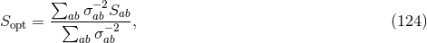
 is a sum over all detector pairs.
In order to perform a search for a given polarization mode one first needs to compute the overlap
reduction functions (using either Eq. (120*) or (121*)) for that mode. With that in hand and a form for the
stochastic background spectrum  , one can construct optimal filters for all pairs in the detector
network using Eq. (119*), and perform the cross-correlations using either Eq. (109*) (or equivalently
Eq. (111*)). Finally, we can calculate the overall network statistic Eq. (124*), by first finding the variances
using Eq. (114*).
, one can construct optimal filters for all pairs in the detector
network using Eq. (119*), and perform the cross-correlations using either Eq. (109*) (or equivalently
Eq. (111*)). Finally, we can calculate the overall network statistic Eq. (124*), by first finding the variances
using Eq. (114*).
It is important to point out that the procedure outlined above is straightforward for ground-based interferometers. However, pulsar timing data are irregularly sampled, and have a pulsar-timing model subtracted out. This needs to be accounted for, and generally, a time-domain approach is more appropriate for these data sets. The procedure is similar to what we have outlined above, but power spectra and gravitational-wave spectra in the frequency domain need to be replaced by auto-covariance and cross-covariance matrices in the time domain that account for the model fitting (for an example of how to do this see [162]).
Interestingly, Nishizawa et al. [329*] show that with three spatially-separated detectors the tensor,
vector, and scalar contributions to the energy density in gravitational waves can be measured
independently. Lee et al. [284] and Alves and Tinto [22] showed that pulsar timing experiments are
especially sensitive to the longitudinal mode, and to a lesser extent the vector modes. Chamberlin and
Siemens [99] showed that the sensitivity of the cross-correlation to the longitudinal mode using
nearby pulsar pairs can be enhanced significantly compared to that of the transverse modes. For
example, for the NANOGrav pulsar timing array, two pulsar pairs separated by  result in
an enhancement of 4 orders of magnitude in sensitivity to the longitudinal mode relative to
the transverse modes. The main contribution to this effect is due to gravitational waves that
are coming from roughly the same direction as the pulses from the pulsars. In this case, the
induced redshift for any gravitational-wave polarization mode is proportional to
result in
an enhancement of 4 orders of magnitude in sensitivity to the longitudinal mode relative to
the transverse modes. The main contribution to this effect is due to gravitational waves that
are coming from roughly the same direction as the pulses from the pulsars. In this case, the
induced redshift for any gravitational-wave polarization mode is proportional to  , the
product of the gravitational-wave frequency and the distance to the pulsar, which can be large.
When the gravitational waves and the pulse direction are exactly parallel, the redshift for the
transverse and vector modes vanishes, but it is proportional to
, the
product of the gravitational-wave frequency and the distance to the pulsar, which can be large.
When the gravitational waves and the pulse direction are exactly parallel, the redshift for the
transverse and vector modes vanishes, but it is proportional to  for the scalar-longitudinal
mode.
for the scalar-longitudinal
mode.
Lee et al. [285] studied the detectability of massive gravitons in pulsar timing arrays through stochastic
background searches. They introduced a modification to Eq. (59*) to account for graviton dispersion, and
found the modified overlap reduction functions (i.e., modifications to the Hellings–Downs curves Eq. (122*))
for various values of the graviton mass. They conclude that a large number of stable pulsars ( ) are
required to distinguish between the massive and massless cases, and that future pulsar timing experiments
could be sensitive to graviton masses of about
) are
required to distinguish between the massive and massless cases, and that future pulsar timing experiments
could be sensitive to graviton masses of about  (
( ). This method is competitive with
some of the compact binary tests described later in Section 5.3.1 (see Table 2). In addition, since the
method of Lee et al. [285] only depends on the form of the overlap reduction functions, it is
advantageous in that it does not involve matched filtering (and therefore prior knowledge of
the waveforms), and generally makes few assumptions about the gravitational-wave source
properties.
). This method is competitive with
some of the compact binary tests described later in Section 5.3.1 (see Table 2). In addition, since the
method of Lee et al. [285] only depends on the form of the overlap reduction functions, it is
advantageous in that it does not involve matched filtering (and therefore prior knowledge of
the waveforms), and generally makes few assumptions about the gravitational-wave source
properties.
 |
 |
 |
Living Rev. Relativity, 16 (2013), 9, doi:10.12942/lrr-2013-9, URL (accessed <date>): http://www.livingreviews.org/lrr-2013-9.
 This work is licensed under a Creative Commons License.
© The author(s), except where otherwise noted.
This work is licensed under a Creative Commons License.
© The author(s), except where otherwise noted.