5 Compact Binary Tests
In this section, we discuss gravitational wave tests of GR with signals emitted by compact binary systems. We begin by explaining the difference between direct and generic tests. We then proceed to describe the many direct or top-down tests and generic or bottom-up tests that have been proposed once gravitational waves are detected, including tests of the no-hair theorems. We concentrate here only on binaries composed of compact objects, such as neutron stars, black holes or other compact exotica. We will not discuss tests one could carry out with electromagnetic information from binary (or double) pulsars, as these are already described in [438*]. We will also not review tests of GR with accretion disk observations, for which we refer the interested reader to [359*].
5.1 Direct and generic tests
Gravitational-wave tests of Einstein’s theory can be classed into two distinct subgroups: direct tests and generic tests. Direct tests employ a top-down approach, where one starts from a particular modified gravity theory with a known action, derives the modified field equations and solves them for a particular gravitational wave-emitting system. On the other hand, generic tests adopt a bottom-up approach, where one takes a particular feature of GR and asks what type of signature its absence would leave on the gravitational-wave observable; one then asks whether the data presents a statistically-significant anomaly pointing to that particular signature.
Direct tests have by far been the traditional approach to testing GR with gravitational waves. The prototypical examples here are tests of Jordan–Fierz–Brans–Dicke theory. As described in Section 2, one can solve the modified field equations for a binary system in the post-Newtonian approximation to find a prediction for the gravitational-wave observable, as we will see in more detail later in this section. Other examples of direct tests include those concerning modified quadratic gravity models and non-commutative geometry theories.
The main advantage of such direct tests is also its main disadvantage: one has to pick a particular modified gravity theory. Because of this, one has a well-defined set of field equations that one can solve, but at the same time, one can only make predictions about that modified gravity model. Unfortunately, we currently lack a particular modified gravity theory that is particularly compelling; many modified gravity theories exist, but none possess all the criteria described in Section 2, except perhaps for the subclass of scalar-tensor theories with spontaneous scalarization. Lacking a clear alternative to GR, it is not obvious which theory one should pick. Given that the full development (from the action to the gravitational wave observable) of any particular theory can be incredibly difficult, time and computationally consuming, carrying out direct tests of all possible modified gravity models once gravitational waves are detected is clearly unfeasible.
Given this, one is led to generic tests of GR, where one asks how the absence of specific features contained in GR could impact the gravitational wave observable. For example, one can ask how such an observable would be modified if the graviton had a mass, if the gravitational interaction were Lorentz or parity violating, or if there existed large extra dimensions. From these general considerations, one can then construct a “meta”-observable, i.e., one that does not belong to a particular theory, but that interpolates over all known possibilities in a well-defined way. This model has come to be known as the parameterized post-Einsteinian framework, in analogy to the parameterized post-Newtonian scheme used to test GR in the solar system [438*]. Given such a construction, one can then ask whether the data points to a statistically-significant deviation from GR.
The main advantage of generic tests is precisely that one does not have to specify a particular model, but instead one lets the data select whether it contains any statistically-significant deviations from our canonical beliefs. Such an approach is, of course, not new to physics, having most recently been successfully employed by the WMAP team [57]. The intrinsic disadvantage of this method is that, if a deviation is found, there is no one-to-one mapping between it and a particular action, but instead one has to point to a class of possible models. Of course, such a disadvantage is not that limiting, since it would provide strong hints as to what type of symmetries or properties of GR would have to be violated in an ultra-violet completion of Einstein’s theory.
5.2 Direct tests
5.2.1 Scalar-tensor theories
Let us first concentrate on Jordan–Fierz–Brans–Dicke theory, where black holes and neutron stars have been shown to exist. In this theory, the gravitational mass depends on the value of the scalar field, as Newton’s constant is effectively promoted to a function, thus leading to violations of the weak-equivalence principle [160, 434, 441*]. The usual prescription for the modeling of binary systems in this theory is due to Eardley [160].8 He showed that such a scalar-field effect can be captured by replacing the constant inertial mass by a function of the scalar field in the distributional stress-energy tensor and then Taylor expanding about the cosmological constant value of the scalar field at spatial infinity, i.e.,
where the subscript![{ ( ) [ ( ) ]} ψ 1 ( ′ 2 ) ψ 2 ψ 3 ma → ma (ϕ) = ma (ϕ0) 1 + saϕ--− 2- sa − sa + sa ϕ-- + 𝒪 ϕ-- , (125 ) 0 0 0](article647x.gif)
 stands for
  different sources, while
  and the sensitivities
  and
and  are defined by
where we remind the reader that
are defined by
where we remind the reader that ![[ ] [ ] ∂ (ln ma ) ′ ∂2 (lnma ) sa ≡ − --------- , sa ≡ − --------2- , (126 ) ∂ (lnG ) 0 ∂ (ln G ) 0](article653x.gif)
 , the derivatives are to be taken with the baryon number held
fixed and evaluated at
, the derivatives are to be taken with the baryon number held
fixed and evaluated at  . These sensitivities encode how the gravitational mass changes due to a
non-constant scalar field; one can think of them as measuring the gravitational binding energy per unit
mass. The internal gravitational field of each body leads to a non-trivial variation of the scalar field, which
then leads to modifications to the gravitational binding energies of the bodies. In carrying out
this expansion, one assumes that the scalar field takes on a constant value at spatial infinity
. These sensitivities encode how the gravitational mass changes due to a
non-constant scalar field; one can think of them as measuring the gravitational binding energy per unit
mass. The internal gravitational field of each body leads to a non-trivial variation of the scalar field, which
then leads to modifications to the gravitational binding energies of the bodies. In carrying out
this expansion, one assumes that the scalar field takes on a constant value at spatial infinity
 , disallowing any homogeneous, cosmological solution to the scalar field evolution equation
[Eq. (19*)].
, disallowing any homogeneous, cosmological solution to the scalar field evolution equation
[Eq. (19*)].
With this at hand, one can solve the massless Jordan–Fierz–Brans–Dicke modified field equations
[Eq. (19*)] for the non-dynamical, near-zone field of  compact objects to obtain [441*]
where  runs from 1 to
  , we have defined the spatial field point distance
  , the
parameterized post-Newtonian quantity
, the
parameterized post-Newtonian quantity  and we have chosen units in
which
and we have chosen units in
which  . This solution is obtained in a post-Newtonian expansion [75*], where the
ellipses represent higher-order terms in
. This solution is obtained in a post-Newtonian expansion [75*], where the
ellipses represent higher-order terms in  and
and  . From such an analysis, one can
also show that compact objects follow geodesics of such a spacetime, to leading order in the
post-Newtonian approximation [160], except that Newton’s constant in the coupling between
matter and gravity is replaced by
. From such an analysis, one can
also show that compact objects follow geodesics of such a spacetime, to leading order in the
post-Newtonian approximation [160], except that Newton’s constant in the coupling between
matter and gravity is replaced by  , in geometric
units.
, in geometric
units.
As is clear from the above analysis, black-hole and neutron-star solutions in this theory generically
depend on the quantities  and
and  . The former determines the strength of the correction, with the
theory reducing to GR in the
. The former determines the strength of the correction, with the
theory reducing to GR in the  limit [164]. The latter depends on the compact object that is
being studied. For neutron stars, this quantity can be computed as follows. First, neglecting scalar
corrections to neutron-star structure and using the Tolman–Oppenheimer–Volkoff equation, one notes that
the mass
limit [164]. The latter depends on the compact object that is
being studied. For neutron stars, this quantity can be computed as follows. First, neglecting scalar
corrections to neutron-star structure and using the Tolman–Oppenheimer–Volkoff equation, one notes that
the mass  , for a fixed equation of state and central density, with
  the total baryon
number. Thus, using Eq. (126*), one has that
the total baryon
number. Thus, using Eq. (126*), one has that
![[ ] sa ≡ 3- 1 − ∂-(ln-ma-) , (131 ) 2 ∂ (ln N ) G](article672x.gif)
 fixed. In this way, given an equation of state and central
density, one can compute the gravitational mass as a function of baryon number, and from this, obtain the
neutron star sensitivities. Eardley [160], Will and Zaglauer [441], and Zaglauer [474*] have shown that these
sensitivities are always in the range
fixed. In this way, given an equation of state and central
density, one can compute the gravitational mass as a function of baryon number, and from this, obtain the
neutron star sensitivities. Eardley [160], Will and Zaglauer [441], and Zaglauer [474*] have shown that these
sensitivities are always in the range  for a soft equation of state and
  for a
stiff one, in both cases monotonically increasing with mass in
for a
stiff one, in both cases monotonically increasing with mass in  . Recently,
Gralla [202] has found a more general method to compute sensitivities is generic modified gravity
theories.
. Recently,
Gralla [202] has found a more general method to compute sensitivities is generic modified gravity
theories.
What is the sensitivity of black holes in generic scalar-tensor theories? Will and Zaglauer [474*] have argued
that the no-hair theorems require  for all black holes, no matter what their mass or spin is. As
already explained in Section 2, stationary black holes that are the byproduct of gravitational collapse (i.e., with
matter that satisfies the energy conditions) in a general class of scalar-tensor theories are identical to their GR
counterparts [224, 408, 159, 398].9
This is because the scalar field satisfies a free wave equation in vacuum, which forces the scalar field to be
constant in the exterior of a stationary, asymptotically-flat spacetime, provided one neglects a homogeneous,
cosmological solution. If the scalar field is to be constant, then by Eq. (127),
for all black holes, no matter what their mass or spin is. As
already explained in Section 2, stationary black holes that are the byproduct of gravitational collapse (i.e., with
matter that satisfies the energy conditions) in a general class of scalar-tensor theories are identical to their GR
counterparts [224, 408, 159, 398].9
This is because the scalar field satisfies a free wave equation in vacuum, which forces the scalar field to be
constant in the exterior of a stationary, asymptotically-flat spacetime, provided one neglects a homogeneous,
cosmological solution. If the scalar field is to be constant, then by Eq. (127),  for a single
black-hole spacetime.
for a single
black-hole spacetime.
Such an argument formally applies only to stationary scenarios, so one might wonder whether a
similar argument holds for binary systems that are in a quasi-stationary arrangement. Will and
Zaglauer [474] and Mirshekari and Will [315] extended this discussion to quasi-stationary spacetimes
describing black-hole binaries to higher post-Newtonian order. They argued that the only possible
deviations from  are due to tidal deformations of the horizon due to the companion,
which are known to arise at very high order in post-Newtonian theory,
are due to tidal deformations of the horizon due to the companion,
which are known to arise at very high order in post-Newtonian theory, ![ψ = 𝒪 [(ma∕ra )5]](article681x.gif) .
Recently, Yunes et al. [465*] extended this argument further by showing that to all orders in
post-Newtonian theory, but in the extreme mass-ratio limit, black holes cannot have scalar hair
in generic scalar-tensor theories. Finally, Healy et al. [230] have carried out a full numerical
simulation of the non-linear field equations, confirming this argument in the full non-linear
regime.
.
Recently, Yunes et al. [465*] extended this argument further by showing that to all orders in
post-Newtonian theory, but in the extreme mass-ratio limit, black holes cannot have scalar hair
in generic scalar-tensor theories. Finally, Healy et al. [230] have carried out a full numerical
simulation of the non-linear field equations, confirming this argument in the full non-linear
regime.
The activation of dynamics in the scalar field for a vacuum spacetime requires either a non-constant
distribution of initial scalar field (violating the constant cosmological scalar field condition at spatial infinity) or
a pure geometrical source to the scalar field evolution equation. The latter would lead to the quadratic
modified gravity theories discussed in Section 2.3.3. As for the former, Horbatsch and Burgess [235] have
argued that if, for example, one lets  , which clearly satisfies
  in a Minkowski
background,10
then a Schwarzschild black hole will acquire modifications that are proportional to
in a Minkowski
background,10
then a Schwarzschild black hole will acquire modifications that are proportional to  . Alternatively, scalar
hair could also be induced by spatial gradients in the scalar field [67], possibly anchored in matter at
galactic scales. Such cosmological hair, however, is likely to be suppressed by a long time scale; in
the example above
. Alternatively, scalar
hair could also be induced by spatial gradients in the scalar field [67], possibly anchored in matter at
galactic scales. Such cosmological hair, however, is likely to be suppressed by a long time scale; in
the example above  must have units of inverse time, and if it is to be associated with the
expansion of the universe, then it would be natural to assume
must have units of inverse time, and if it is to be associated with the
expansion of the universe, then it would be natural to assume  , where
  is the
Hubble parameter. Therefore, although such cosmological hair might have an effect on black
holes in the early universe, it should not affect black hole observations at moderate to low
redshifts.
is the
Hubble parameter. Therefore, although such cosmological hair might have an effect on black
holes in the early universe, it should not affect black hole observations at moderate to low
redshifts.
Scalar field dynamics can be activated in non-vacuum spacetimes, even if initially the stars are not scalarized provided one considers a more general scalar-tensor theory, like the one introduced by Damour and Esposito-Farèse [129*, 130*]. As discussed in Section 2.3.1, when the conformal factor takes on a particular functional form, non-linear effects induced when the gravitational energy exceeds a certain threshold can spontaneously scalarize merging neutron stars, as demonstrated recently by Barausse, et al [51*]. Therefore, neutron stars in binaries are likely to have hair in generic scalar-tensor theories, even if they start their inspiral unscalarized.
What do gravitational waves look like in Jordan–Fierz–Brans–Dicke theory? As described in
Section 2.3.1, both the scalar field perturbation  and the new metric perturbation
  satisfy a sourced wave equation [Eq. (19*)], whose leading-order solution for a two-body inspiral
is [436*]
satisfy a sourced wave equation [Eq. (19*)], whose leading-order solution for a two-body inspiral
is [436*]
where  is the distance to the detector,
  is a unit vector pointing toward the detector,
  is the
magnitude of relative position vector
is the
magnitude of relative position vector  , with
  the trajectory of body
  ,
,  is the reduced mass and
  is the total mass,
  is the relative velocity vector and
we have defined the shorthands
is the relative velocity vector and
we have defined the shorthands
We have also introduced multi-index notation here, such that  . Such a solution is
derived using the Lorenz gauge condition
. Such a solution is
derived using the Lorenz gauge condition  and in a post-Newtonian expansion, where we have
left out subleading terms of relative order
and in a post-Newtonian expansion, where we have
left out subleading terms of relative order  or
or  .
.
Given the new metric perturbation  , one can reconstruct the gravitational wave
  metric
perturbation, and from this, the response function, associated with the quasi-circular inspiral of compact
binaries. After using Kepler’s third law to simplify expressions [
metric
perturbation, and from this, the response function, associated with the quasi-circular inspiral of compact
binaries. After using Kepler’s third law to simplify expressions [ , where
  is the orbital
angular frequency and
is the orbital
angular frequency and  is the total mass and
  is the orbital separation], one finds for a ground-based
L-shaped detector [102*]:
is the orbital separation], one finds for a ground-based
L-shaped detector [102*]:
where  is the symmetric mass ratio,
  is the chirp mass,
  is the
inclination angle, and where we have used the beam-pattern functions in Eq. (58*). In Eq. (136) and
henceforth, we linearize all expressions in
is the
inclination angle, and where we have used the beam-pattern functions in Eq. (58*). In Eq. (136) and
henceforth, we linearize all expressions in  . Jordan–Fierz–Brans–Dicke theory predicts the
generic excitation of three polarizations: the usual plus and cross polarizations, and a breathing,
scalar mode. We see that the latter contributes to the response at two, one and zero times the
orbital frequency. One should note that all of these corrections arise during the generation of
gravitational waves, and not due to a propagation effect. In fact, gravitational waves travel at
the speed of light (and the graviton remains massless) in standard Jordan–Fierz–Brans–Dicke
theory.
. Jordan–Fierz–Brans–Dicke theory predicts the
generic excitation of three polarizations: the usual plus and cross polarizations, and a breathing,
scalar mode. We see that the latter contributes to the response at two, one and zero times the
orbital frequency. One should note that all of these corrections arise during the generation of
gravitational waves, and not due to a propagation effect. In fact, gravitational waves travel at
the speed of light (and the graviton remains massless) in standard Jordan–Fierz–Brans–Dicke
theory.
The quantities  and
and  are the orbital phase and frequency respectively, which are to be found by
solving the differential equation
are the orbital phase and frequency respectively, which are to be found by
solving the differential equation
![2∕5 [ ( 2 ) ] dF-= (1 − γ)S2 η---ℳ −2(2πℳcF )3 + 48-ℳ −2(2π ℳcF )11∕3 1 − 1 −-γ- 1 − Γ--+ 4S2 ...(,137 ) dt π c 5π c 2 6 3](article720x.gif)
![[ ( ) ] 2 2 2m4 2 32 2 2( m )5 1 − γ Γ 2 E˙BD = − --𝒢12η --4 (1 − γ )S − ---𝒢12η -- 1 − ------ 1 − --- + ..., (138 ) 3 r 5 r 2 6](article721x.gif)
 , one finds
where we have defined  . In deriving these equations, we have neglected the last term
in Eq. (137*), as this is a constant that can be reabsorbed into the chirp mass. Notice that since the two
definitions of chirp mass differ only by a term of
. In deriving these equations, we have neglected the last term
in Eq. (137*), as this is a constant that can be reabsorbed into the chirp mass. Notice that since the two
definitions of chirp mass differ only by a term of  , the first term of Eq. (137*) is not
modified.
, the first term of Eq. (137*) is not
modified.
One of the main ingredients that goes into parameter estimation is the Fourier transform of the response function. This can be estimated in the stationary-phase approximation, for a simple, non-spinning, quasi-circular inspiral. In this approximation, one assumes the phase is changing much more rapidly than the amplitude [56*, 125*, 153*, 457*]. One finds [102*]

where we have defined the amplitudes
and the Fourier phase
where the Brans–Dicke correction is kept only to leading order in  and
and  , while
  are
post-Newtonian GR coefficients (see, e.g., [265]). In writing the Fourier response in this way, we had to
redefine the phase of coalescence via
are
post-Newtonian GR coefficients (see, e.g., [265]). In writing the Fourier response in this way, we had to
redefine the phase of coalescence via

where  is the Kronecker delta and
  is the GR phase of coalescence (defined as an integration
constant when the frequency diverges). Of course, in this calculation we have neglected amplitude
corrections that arise purely in GR, if one were to carry out the post-Newtonian approximation to higher
order.
is the GR phase of coalescence (defined as an integration
constant when the frequency diverges). Of course, in this calculation we have neglected amplitude
corrections that arise purely in GR, if one were to carry out the post-Newtonian approximation to higher
order.
Many studies have been carried out to determine the level at which such corrections to the waveform
could be measured or constrained once a gravitational wave has been detected. The first such study was
carried out by Will [436*], who determined that given a LIGO detection at SNR  of a
of a
 black-hole/neutron-star non-spinning, quasi-circular inspiral, one could constrain
 . Scharre and Will [379*] carried out a similar analysis but for a LISA detection
with
. Scharre and Will [379*] carried out a similar analysis but for a LISA detection
with  of a
of a  intermediate-mass black-hole/neutron-star, non-spinning,
quasi-circular inspiral, and found that one could constrain
intermediate-mass black-hole/neutron-star, non-spinning,
quasi-circular inspiral, and found that one could constrain  . Such an analysis was
then repeated by Will and Yunes [440*] but as a function of the classic LISA instrument. They
found that the bound is independent of the LISA arm length, but inversely proportional to the
LISA position noise error, if the position error noise dominates over laser shot noise. All such
studies considered an angle-averaged signal that neglected the spin of either body, assumptions
that were relaxed by Berti et al. [63*, 64]. They carried out Monte-Carlo simulations over all
signal sky positions that included spin-orbit precession to find that the projected bound with
LISA deteriorates to
. Such an analysis was
then repeated by Will and Yunes [440*] but as a function of the classic LISA instrument. They
found that the bound is independent of the LISA arm length, but inversely proportional to the
LISA position noise error, if the position error noise dominates over laser shot noise. All such
studies considered an angle-averaged signal that neglected the spin of either body, assumptions
that were relaxed by Berti et al. [63*, 64]. They carried out Monte-Carlo simulations over all
signal sky positions that included spin-orbit precession to find that the projected bound with
LISA deteriorates to  for the same system and SNR. This was confirmed and
extended by Yagi et al. [450*], who in addition to spin-orbit precession allowed for non-circular
(eccentric) inspirals. In fact, when eccentricity is included, the bound deteriorates even further to
for the same system and SNR. This was confirmed and
extended by Yagi et al. [450*], who in addition to spin-orbit precession allowed for non-circular
(eccentric) inspirals. In fact, when eccentricity is included, the bound deteriorates even further to
 . The same authors also found that similar gravitational-wave observations
with the next-generation detector DECIGO could constrain
. The same authors also found that similar gravitational-wave observations
with the next-generation detector DECIGO could constrain  . Similarly, for a
non-spinning neutron-star/black-hole binary, the future ground-based detector, the Einstein Telescope
(ET) [361], could place constraints about 5 times stronger than the Cassini bound, as shown
in [38*].
. Similarly, for a
non-spinning neutron-star/black-hole binary, the future ground-based detector, the Einstein Telescope
(ET) [361], could place constraints about 5 times stronger than the Cassini bound, as shown
in [38*].
All such projected constraints are to be compared with the current solar system bound of  placed through the tracking of the Cassini spacecraft [73*]. Table 1 presents all such bounds for ease of
comparison,11
normalized to an SNR of 10. As should be clear, it is unlikely that LIGO observations will be able to
constrain
placed through the tracking of the Cassini spacecraft [73*]. Table 1 presents all such bounds for ease of
comparison,11
normalized to an SNR of 10. As should be clear, it is unlikely that LIGO observations will be able to
constrain  better than current solar system bounds. In fact, even LISA would probably not
be able to do better than the Cassini bound. Table 1 also shows that the inclusion of more
complexity in the waveform seems to dilute the level at which
better than current solar system bounds. In fact, even LISA would probably not
be able to do better than the Cassini bound. Table 1 also shows that the inclusion of more
complexity in the waveform seems to dilute the level at which  can be constrained. This is
because the inclusion of eccentricity and spin forces one to introduce more parameters in the
waveform, without these modifications truly adding enough waveform complexity to break
the induced degeneracies. One would then expect that the inclusion of amplitude modulation
due to precession and higher harmonics should break such degeneracies, at least partially, as
was found for massive black-hole binary [279, 280]. However, even then it seems reasonable to
expect that only third-generation detectors will be able to constrain
can be constrained. This is
because the inclusion of eccentricity and spin forces one to introduce more parameters in the
waveform, without these modifications truly adding enough waveform complexity to break
the induced degeneracies. One would then expect that the inclusion of amplitude modulation
due to precession and higher harmonics should break such degeneracies, at least partially, as
was found for massive black-hole binary [279, 280]. However, even then it seems reasonable to
expect that only third-generation detectors will be able to constrain  beyond solar-system
levels.
beyond solar-system
levels.
| Reference | Binary mass | ![4 ωBD [10 ]](article748x.gif) |
Properties |
| [73] | x | 4 | Solar system |
| [436*] |  |
0.1 | LIGO, Fisher, Ang. Ave. |
| circular, non-spinning | |||
| [379] |  |
24 | LISA, Fisher, Ang. Ave. |
| circular, non-spinning | |||
| [440*] |  |
20 | LISA, Fisher, Ang. Ave. |
| circular, non-spinning | |||
| [63*] |  |
0.7 | LISA, Fisher, Monte-Carlo |
| circular, w/spin-orbit | |||
| [450*] |  |
0.5 | LISA, Fisher, Monte-Carlo |
| eccentric, spin-orbit | |||
| [451*] |  |
160 | DECIGO, Fisher, Monte-Carlo |
| eccentric, spin-orbit | |||
| [38] |  |
10 | ET, Fisher, Ang. Ave. |
| circular, non-spinning | |||
The main reason that solar-system constraints of Jordan–Fierz–Brans–Dicke theory cannot be beaten with gravitational-wave observations is that the former are particularly well-suited to constrain weak-field deviations of GR. One might have thought that scalar-tensor theories constitute strong-field tests of Einstein’s theory, but this is not quite true, as argued in Section 2.3.1. One can see this clearly by noting that scalar-tensor theory predicts dipolar radiation, which dominates at low velocities over the GR prediction (precisely the opposite behavior that one would expect from a strong-field modification to Einstein’s theory).
However, one should note that all the above analysis considered only the inspiral phase of
coalescence, usually truncating their study at the innermost stable-circular orbit. The merger and
ringdown phases, where most of the gravitational wave power resides, have so far been mostly
neglected. One might expect that an increase in power will be accompanied by an increase in SNR,
thus allowing us to constrain  further, as this scales with 1/SNR [262*]. Moreover, during
merger and ringdown, dynamical strong-field gravity effects in scalar-tensor theories could affect
neutron star parameters and their oscillations [395], as well as possibly induce spontaneous
scalarization [51*]. All of these non-linear effects could easily lead to a strengthening of projected
bounds. However, to date no detailed analysis has attempted to determine how well one could
constrain scalar-tensor theories using full information about the entire coalescence of a compact
binary.
further, as this scales with 1/SNR [262*]. Moreover, during
merger and ringdown, dynamical strong-field gravity effects in scalar-tensor theories could affect
neutron star parameters and their oscillations [395], as well as possibly induce spontaneous
scalarization [51*]. All of these non-linear effects could easily lead to a strengthening of projected
bounds. However, to date no detailed analysis has attempted to determine how well one could
constrain scalar-tensor theories using full information about the entire coalescence of a compact
binary.
The subclass of scalar-tensor models described by Jordan–Fierz–Brans–Dicke theory is not the only type
of model that can be constrained with gravitational-wave observations. In the extreme–mass-ratio limit, for
binaries consisting of a stellar-mass compact object spiraling into a supermassive black hole, Yunes et
al. [465*] have recently shown that generic scalar-tensor theories reduce to either massless or massive
Jordan–Fierz–Brans–Dicke theory. Of course, in this case the sensitivities need to be calculated from the
equations of structure within the full scalar-tensor theory. The inclusion of a scalar field mass leads to an
interesting possibility: floating orbits [94*]. Such orbits arise when the small compact object
experiences superradiance, leading to resonances in the scalar flux that can momentarily counteract
the gravitational-wave flux, leading to a temporarily-stalled orbit that greatly modifies the
orbital-phase evolution. These authors showed that if an extreme mass-ratio inspiral is detected with a
template consistent with GR, this alone allows us to rule out a large region of  phase
space, where
phase
space, where  is the mass of the scalar (see Figure 1 in [465*]). This is because if such an
inspiral had gone through a resonance, a GR template would be grossly different from the signal.
Such bounds are dramatically stronger than the current most stringent bound
is the mass of the scalar (see Figure 1 in [465*]). This is because if such an
inspiral had gone through a resonance, a GR template would be grossly different from the signal.
Such bounds are dramatically stronger than the current most stringent bound  and
and  obtained from Cassini measurements of the Shapiro time-delay
in the solar system [20*]. Even if resonances are not hit, Berti et al. [71] have estimated that
second-generation ground-based interferometers could constrain the combination
obtained from Cassini measurements of the Shapiro time-delay
in the solar system [20*]. Even if resonances are not hit, Berti et al. [71] have estimated that
second-generation ground-based interferometers could constrain the combination  with the observation of gravitational waves from neutron-star/binary inspirals at an SNR of
 . These bounds can also be stronger than current constraints, especially for large scalar
mass.
. These bounds can also be stronger than current constraints, especially for large scalar
mass.
Lastly one should mention possible gravitational-wave constraints on other types of scalar tensor theories. Let us first consider Brans–Dicke type scalar-tensor theories, where the coupling constant is allowed to vary. Will [436] has argued that the constraints described in Table 1 go through, with the change
where![[ ] -2𝒢1,2-- -2𝒢1,2-- ---2-ω′BD---- 2 2 + ω → 2 + ω 1 + (3 + 2ω )2 , (146 ) BD BD BD](article763x.gif)
 . In the
  limit, this implies the replacement
 ![ωBD → ωBD [1 + ω ′BD∕(2ω2BD)]−2](article766x.gif) .
Of course, this assumes that there is neither a potential nor a geometric source driving the
evolution of the scalar field, and is not applicable for theories where spontaneous scalarization is
present [129*].
.
Of course, this assumes that there is neither a potential nor a geometric source driving the
evolution of the scalar field, and is not applicable for theories where spontaneous scalarization is
present [129*].
Another interesting scalar-tensor theory to consider is that studied by Damour and
Esposito-Farèse [129, 130]. As explained in Section 2.3.1, this theory is defined by the action of Eq. (14*)
with the conformal factor  . In standard Brans–Dicke theory, only mixed binaries composed
of a black hole and a neutron star lead to large deviations from GR due to dipolar emission.
This is because dipole emission is proportional to the difference in sensitivities of the binary
components. For neutron–star binaries with similar masses, this difference is close to zero, while for
black holes it is identically zero (see Eqs. (134) and (144)). However, in the theory considered
by Damour and Esposito-Farèse , when the gravitational energy is large enough, as in the
very late inspiral, non-linear effects can lead to drastic modifications from the GR expectation,
such as spontaneous scalarization [51]. Unfortunately, most of this happens at rather high
frequency, and thus, it is not clear whether such effects are observable with current ground-based
detectors.
. In standard Brans–Dicke theory, only mixed binaries composed
of a black hole and a neutron star lead to large deviations from GR due to dipolar emission.
This is because dipole emission is proportional to the difference in sensitivities of the binary
components. For neutron–star binaries with similar masses, this difference is close to zero, while for
black holes it is identically zero (see Eqs. (134) and (144)). However, in the theory considered
by Damour and Esposito-Farèse , when the gravitational energy is large enough, as in the
very late inspiral, non-linear effects can lead to drastic modifications from the GR expectation,
such as spontaneous scalarization [51]. Unfortunately, most of this happens at rather high
frequency, and thus, it is not clear whether such effects are observable with current ground-based
detectors.
5.2.2 Modified quadratic gravity
Black holes exist in the classes of modified quadratic gravity that have so far been considered. In
non-dynamical theories (when  and the scalar-fields are constant, refer to Eq. (25)), Stein and
Yunes [473*] have shown that all metrics that are Ricci tensor flat are also solutions to the modified field
equations (see also [360*]). This is not so for dynamical theories, since then the
and the scalar-fields are constant, refer to Eq. (25)), Stein and
Yunes [473*] have shown that all metrics that are Ricci tensor flat are also solutions to the modified field
equations (see also [360*]). This is not so for dynamical theories, since then the  field is sourced by
curvature, leading to corrections to the field equations proportional to the Riemann tensor and its
dual.
field is sourced by
curvature, leading to corrections to the field equations proportional to the Riemann tensor and its
dual.
In dynamical Chern–Simons gravity, stationary and spherically-symmetric spacetimes are still described by GR solutions, but stationary and axisymmetric spacetimes are not. Instead, they are represented by [466*, 272*]
with the scalar field where

 is the line element of the Kerr metric and we recall that
  in the notation
of Section 2.3.3. These expressions are obtained in Boyer–Lindquist coordinates and in the
small-rotation/small-coupling limit to
in the notation
of Section 2.3.3. These expressions are obtained in Boyer–Lindquist coordinates and in the
small-rotation/small-coupling limit to  in [466*, 272] and to
  in [455]. The
linear-in-spin corrections modify the frame-dragging effect and they are of 3.5 post-Newtonian order. The
quadratic-in-spin corrections modify the quadrupole moment, which induces 2 post-Newtonian-order
corrections to the binding energy. However, the stability of these black holes has not yet been
demonstrated.
in [455]. The
linear-in-spin corrections modify the frame-dragging effect and they are of 3.5 post-Newtonian order. The
quadratic-in-spin corrections modify the quadrupole moment, which induces 2 post-Newtonian-order
corrections to the binding energy. However, the stability of these black holes has not yet been
demonstrated.
In Einstein-Dilaton-Gauss–Bonnet gravity, stationary and spherically-symmetric spacetimes are described, in the small-coupling approximation, by the line element [473*]
in Schwarzschild coordinates, where
 is the line element on the two-sphere,
  is the
Schwarzschild factor and we have defined
is the
Schwarzschild factor and we have defined
while the corresponding scalar field is
This solution is not restricted just to Einstein-Dilaton-Gauss–Bonnet gravity, but it is also the most general, stationary and spherically-symmetric solution in quadratic gravity. This is because all terms proportional to
 are proportional to the Ricci tensor, which vanishes in vacuum GR, while the
  term does not
contribute in spherical symmetry (see [473*] for more details). Linear slow-rotation corrections to this
solution have been found in [345]. Although the stability of these black holes has not yet been
demonstrated, other dilatonic black hole solutions obtained numerically (equivalent to those in
Einstein-Dilaton-Gauss–Bonnet theory in the limit of small fields) [257] have been found to be stable under
axial perturbations [258, 409, 343].
term does not
contribute in spherical symmetry (see [473*] for more details). Linear slow-rotation corrections to this
solution have been found in [345]. Although the stability of these black holes has not yet been
demonstrated, other dilatonic black hole solutions obtained numerically (equivalent to those in
Einstein-Dilaton-Gauss–Bonnet theory in the limit of small fields) [257] have been found to be stable under
axial perturbations [258, 409, 343].
Neutron stars also exist in quadratic modified gravity. In dynamical Chern–Simons gravity, the mass-radius relation remains unmodified to first order in the slow-rotation expansion, but the moment of inertia changes to this order [469, 19*], while the quadrupole moment and the mass measured at spatial infinity change to quadratic order in spin [448*]. This is because the mass-radius relation, to first order in slow-rotation, depends on the spherically-symmetric part of the metric, which is unmodified in dynamical Chern–Simons gravity. In Einstein-Dilaton-Gauss–Bonnet gravity, the mass-radius relation is modified [342*]. As in GR, these functions must be solved for numerically and they depend on the equation of state.
Gravitational waves are also modified in quadratic modified gravity. In dynamical Chern–Simons gravity, Garfinkle et al. [190] have shown that the propagation of such waves on a Minkowski background remains unaltered, and thus, all modifications arise during the generation stage. In Einstein-Dilaton-Gauss–Bonnet theory, no such analysis of the propagation of gravitational waves has yet been carried out. Yagi et al. [447*] studied the generation mechanism in both theories during the quasi-circular inspiral of comparable-mass, spinning black holes in the post-Newtonian and small-coupling approximations. They found that a standard post-Newtonian analysis fails for such theories because the assumption that black holes can be described by a distributional stress-energy tensor without any further structure fails. They also found that since black holes acquire scalar hair in these theories, and this scalar field is anchored to the curvature profiles, as black holes move, the scalar fields must follow the singularities, leading to dipole scalar-field emission.
During a quasi-circular inspiral of spinning black holes in dynamical Chern–Simons gravity, the total gravitational wave energy flux carried out to spatial infinity (equal to minus the rate of change of a binary’s binding energy by the balance law) is modified from the GR expectation to leading order by [447*]
due to scalar field radiation and corrections to the metric perturbation that are of magnetic-type, quadrupole form. In this equation,![˙CS { ⟨ ⟩ } δEspin-= ζη −2 -25--[¯Δ + 2⟨(Δ¯ ⋅ ˆv )⟩] + 75a1a2- ˆSiˆSj (2ˆvi ˆvj − 2ˆni ˆnj ) v4 , (153 ) E˙GR 4 1536 12 16 m2 1 2 12 12 12 12 12](article783x.gif)
 is the leading-order GR prediction for the total
energy flux,
is the leading-order GR prediction for the total
energy flux,  is the dimensionless Chern–Simons coupling parameter,
  is the
magnitude of the relative velocity with unit vector
is the
magnitude of the relative velocity with unit vector  ,
,  ,
where
,
where  is the Kerr spin parameter of the
  th black hole and
  is the unit vector in the direction
of the spin angular momentum, the unit vector
is the unit vector in the direction
of the spin angular momentum, the unit vector  points from body one to two, and the
angle brackets stand for an average over several gravitational wave wavelengths. If the black
holes are not spinning, then the correction to the scalar energy flux is greatly suppressed [447*]
where we have defined the reduced mass difference
points from body one to two, and the
angle brackets stand for an average over several gravitational wave wavelengths. If the black
holes are not spinning, then the correction to the scalar energy flux is greatly suppressed [447*]
where we have defined the reduced mass difference 
 . Notice that this is a 7
post-Newtonian–order correction , instead of a 2 post-Newtonian correction as in Eq. (153*). In the
non-spinning limit, the dynamical Chern–Simons correction to the metric tensor induces a 6
post-Newtonian–order correction to the gravitational energy flux [447*], which is consistent with the
numerical results of [344].
. Notice that this is a 7
post-Newtonian–order correction , instead of a 2 post-Newtonian correction as in Eq. (153*). In the
non-spinning limit, the dynamical Chern–Simons correction to the metric tensor induces a 6
post-Newtonian–order correction to the gravitational energy flux [447*], which is consistent with the
numerical results of [344].
On the other hand, in Einstein-Dilaton-Gauss–Bonnet gravity, the corrections to the energy flux are [447*]
which is a
 post-Newtonian correction. This is because the scalar field
  behaves like a
monopole (see Eq. (152*)), and when such a scalar monopole is dragged by the black hole, it emits
electric-type, dipole scalar radiation. Any hairy black hole with monopole hair will thus emit dipolar
radiation, leading to
behaves like a
monopole (see Eq. (152*)), and when such a scalar monopole is dragged by the black hole, it emits
electric-type, dipole scalar radiation. Any hairy black hole with monopole hair will thus emit dipolar
radiation, leading to  post-Newtonian corrections in the energy flux carried to spatial
infinity.
post-Newtonian corrections in the energy flux carried to spatial
infinity.
Such modifications to the energy flux modify the rate of change of the binary’s binding energy through
the balance law,  , which in turn modify the rate of change of the gravitational wave frequency
and phase,
, which in turn modify the rate of change of the gravitational wave frequency
and phase,  . For dynamical Chern–Simons gravity (when the spins are aligned with
the orbital angular momentum) and for Einstein-Dilaton-Gauss–Bonnet theory (in the non-spinning case),
the Fourier transform of the gravitational-wave response function in the stationary phase approximation
becomes [447*, 454*]
. For dynamical Chern–Simons gravity (when the spins are aligned with
the orbital angular momentum) and for Einstein-Dilaton-Gauss–Bonnet theory (in the non-spinning case),
the Fourier transform of the gravitational-wave response function in the stationary phase approximation
becomes [447*, 454*]

 is the Fourier transform of the response in GR,
  with
with  the gravitational
wave frequency and [447*, 454*]
the gravitational
wave frequency and [447*, 454*]
where we have defined the symmetric and antisymmetric spin combinations
 . We have here neglected any possible amplitude correction, but we have
included both deformations to the binding energy and Kepler’s third law, in addition to changes in the
energy flux, when computing the phase correction. However, in Einstein-Dilaton-Gauss–Bonnet theory the
binding energy is modified at higher post-Newtonian order, and thus, corrections to the energy flux control
the modifications to the gravitational-wave response function.
. We have here neglected any possible amplitude correction, but we have
included both deformations to the binding energy and Kepler’s third law, in addition to changes in the
energy flux, when computing the phase correction. However, in Einstein-Dilaton-Gauss–Bonnet theory the
binding energy is modified at higher post-Newtonian order, and thus, corrections to the energy flux control
the modifications to the gravitational-wave response function.
From the above analysis, it should be clear that the corrections to the gravitational-wave observable in
quadratic modified gravity are always proportional to the quantity  . Thus,
any measurement that is consistent with GR will allow a constraint of the form
. Thus,
any measurement that is consistent with GR will allow a constraint of the form  , where
  is a
number of order unity, and
is a
number of order unity, and  is the accuracy of the measurement. Solving for the coupling constants of
the theory, such a measurement would lead to
is the accuracy of the measurement. Solving for the coupling constants of
the theory, such a measurement would lead to  [390*]. Therefore, constraints on
quadratic modified gravity will weaken for systems with larger characteristic mass. This can be
understood by noticing that the corrections to the action scale with positive powers of the Riemann
tensor, while this scales inversely with the mass of the object, i.e., the smaller a compact object
is, the larger its curvature. Such an analysis then automatically predicts that LIGO will be
able to place stronger constraints than LISA-like missions on such theories, because LIGO
operates in the 100 Hz frequency band, allowing for the detection of stellar-mass inspirals,
while LISA-like missions operate in the mHz band, and are limited to supermassive black-holes
inspirals.
[390*]. Therefore, constraints on
quadratic modified gravity will weaken for systems with larger characteristic mass. This can be
understood by noticing that the corrections to the action scale with positive powers of the Riemann
tensor, while this scales inversely with the mass of the object, i.e., the smaller a compact object
is, the larger its curvature. Such an analysis then automatically predicts that LIGO will be
able to place stronger constraints than LISA-like missions on such theories, because LIGO
operates in the 100 Hz frequency band, allowing for the detection of stellar-mass inspirals,
while LISA-like missions operate in the mHz band, and are limited to supermassive black-holes
inspirals.
How well can these modifications be measured with gravitational-wave observations? Yagi et al. [447*]
predicted, based on the results of Cornish et al. [124*], that a sky-averaged LIGO gravitational-wave
observation with SNR of 10 of the quasi-circular inspiral of non-spinning black holes with masses
 would allow a constraint of
  , where we recall that
  . A similar
sky-averaged, eLISA observation of a quasi-circular, spin-aligned black-hole inspiral with masses
. A similar
sky-averaged, eLISA observation of a quasi-circular, spin-aligned black-hole inspiral with masses
 would constrain
  [447]. The loss in constraining power comes
from the fact that the constraint on
[447]. The loss in constraining power comes
from the fact that the constraint on  will scale with the total mass of the binary, which
is six orders of magnitude larger for space-borne sources. These constraints are not stronger
than current bounds from the existence of compact objects [342] (
will scale with the total mass of the binary, which
is six orders of magnitude larger for space-borne sources. These constraints are not stronger
than current bounds from the existence of compact objects [342] ( ) and from the
change in the orbital period of the low-mass x-ray binary A0620–00 (
) and from the
change in the orbital period of the low-mass x-ray binary A0620–00 ( ) [444], but
they are independent of the nature of the object and sample the theory in a different energy
scale. In dynamical Chern–Simons gravity, one expects similar projected gravitational-wave
constraints on
) [444], but
they are independent of the nature of the object and sample the theory in a different energy
scale. In dynamical Chern–Simons gravity, one expects similar projected gravitational-wave
constraints on  , namely
  , where
  is the total mass of the binary system in
kilometers. Therefore, for binaries detectable with ground-based interferometers, one expects
constraints of order
is the total mass of the binary system in
kilometers. Therefore, for binaries detectable with ground-based interferometers, one expects
constraints of order  . In this case, such a constraint would be roughly six orders of
magnitude stronger than current LAGEOS bounds [19]. Dynamical Chern–Simons gravity
cannot be constrained with binary pulsar observations, since the theory’s corrections to the
post-Keplerian observables are too high post-Newtonian order, given the current observational
uncertainties [448]. However, the gravitational wave constraint is more difficult to achieve in the dynamical
Chern–Simons case, because the correction to the gravitational wave phase is degenerate with spin.
However, Yagi et al. [454*] argued that precession should break this degeneracy, and if a signal
with sufficiently high SNR is observed, such bounds would be possible. One must be careful, of
course, to check that the small-coupling approximation is still satisfied when saturating such a
constraint [454].
. In this case, such a constraint would be roughly six orders of
magnitude stronger than current LAGEOS bounds [19]. Dynamical Chern–Simons gravity
cannot be constrained with binary pulsar observations, since the theory’s corrections to the
post-Keplerian observables are too high post-Newtonian order, given the current observational
uncertainties [448]. However, the gravitational wave constraint is more difficult to achieve in the dynamical
Chern–Simons case, because the correction to the gravitational wave phase is degenerate with spin.
However, Yagi et al. [454*] argued that precession should break this degeneracy, and if a signal
with sufficiently high SNR is observed, such bounds would be possible. One must be careful, of
course, to check that the small-coupling approximation is still satisfied when saturating such a
constraint [454].
5.2.3 Non-commutative geometry
Black holes exist in non-commutative geometry theories, as discussed in Section 2.3.5. What is more, the
usual Schwarzschild and Kerr solutions of GR persist in these theories. This is not because
such solutions have vanishing Weyl tensor, but because the quantity  happens to
vanish for such metrics. Similarly, one would expect that the two-body, post-Newtonian metric
that describes a black-hole–binary system should also satisfy the non-commutative geometry
field equations, although this has not been proven explicitly. Similarly, although neutron-star
spacetimes have not yet been considered in non-commutative geometries, it is likely that if such
spacetimes are stationary and satisfy the Einstein equations, they will also satisfy the modified field
equations. Much more work on this is still needed to establish all of these concepts on a firmer
basis.
happens to
vanish for such metrics. Similarly, one would expect that the two-body, post-Newtonian metric
that describes a black-hole–binary system should also satisfy the non-commutative geometry
field equations, although this has not been proven explicitly. Similarly, although neutron-star
spacetimes have not yet been considered in non-commutative geometries, it is likely that if such
spacetimes are stationary and satisfy the Einstein equations, they will also satisfy the modified field
equations. Much more work on this is still needed to establish all of these concepts on a firmer
basis.
Gravitational waves exist in non-commutative gravity. Their generation for a compact binary system in a circular orbit was analyzed by Nelson et al., in [326*, 325*]. They began by showing that a transverse-traceless gauge exists in this theory, although the transverse-traceless operator is slightly different from that in GR. They then proceeded to solve the modified field equations for the metric perturbation [Eq. (42*)] via a Green’s function approach:
where recall that
 acts like a mass term, the integral is taken over the entire past light
cone,
acts like a mass term, the integral is taken over the entire past light
cone,  is the Bessel function of the first kind,
  is the distance from the source to the observer and
the quadrupole moment is defined as usual:
where
is the distance from the source to the observer and
the quadrupole moment is defined as usual:
where 
 is the time-time component of the matter stress-energy tensor. Of course, this is only the first
term in an infinite multipole expansion.
is the time-time component of the matter stress-energy tensor. Of course, this is only the first
term in an infinite multipole expansion.
Although the integral in Eq. (159*) has not yet been solved in the post-Newtonian approximation, Nelson et al. [326*, 325*] did solve for its time derivative to find
where  is the orbital angular frequency and we have defined
and one has assumed that the binary is in the  -
- plane and the observer is on the
  -axis.
However, if one expands these expressions about
-axis.
However, if one expands these expressions about  , one recovers the GR solution to leading
order, plus corrections that decay faster than
, one recovers the GR solution to leading
order, plus corrections that decay faster than  . This then automatically implies that such
modifications to the generation mechanism will be difficult to observe for sources at astronomical
distances.
. This then automatically implies that such
modifications to the generation mechanism will be difficult to observe for sources at astronomical
distances.
Given such a solution, one can compute the flux of energy carried by gravitational waves to spatial infinity. Stein and Yunes [400*] have shown that in quadratic gravity theories, this flux is still given by
where
 is the trace-reversed metric perturbation, the integral is taken over a 2-sphere at spatial
infinity, and we recall that the angle brackets stand for an average over several wavelengths. Given the
solution in Eq. (161), one finds that the energy flux is
The asymptotic expansion of the term in between square brackets about
is the trace-reversed metric perturbation, the integral is taken over a 2-sphere at spatial
infinity, and we recall that the angle brackets stand for an average over several wavelengths. Given the
solution in Eq. (161), one finds that the energy flux is
The asymptotic expansion of the term in between square brackets about ![[ ( ) ( ) ] E˙= -9μ2r2 Ω4 β2 |r |2f2 β |r|, 2Ω + |r|2f2 β |r|, 2Ω . (165 ) 20 12 c β s β](article841x.gif)
 is
which then leads to an energy flux identical to that in GR, as any subdominant term goes to zero when the
2-sphere of integration is taken to spatial infinity. In that case, there are no modifications to the rate of
change of the orbital frequency. Of course, if one were not to expand about
is
which then leads to an energy flux identical to that in GR, as any subdominant term goes to zero when the
2-sphere of integration is taken to spatial infinity. In that case, there are no modifications to the rate of
change of the orbital frequency. Of course, if one were not to expand about ![[ ( ) ( ) ] { [ ( )]} 2 2 2Ω- 2 2Ω- 2 --1--- -1- |r| fc β|r|, β + fs β |r|, β ∼ |r| β2|r|2 1 + 𝒪 |r| , (166 )](article843x.gif)
 , then the energy flux
would lead to certain resonances at
, then the energy flux
would lead to certain resonances at  , but the energy flux is only well-defined at future null
infinity.
, but the energy flux is only well-defined at future null
infinity.
The above analysis was used by Nelson et al. [326*, 325*] to compute the rate of change of the orbital
period of binary pulsars, in the hopes of using this to constrain  . Using data from the binary
pulsar, they stipulated an order-of-magnitude constraint of
. Using data from the binary
pulsar, they stipulated an order-of-magnitude constraint of  . However, such an
analysis could be revisited to relax a few assumptions used in [326*, 325*]. First, binary pulsar
constraints on modified gravity theories require the use of at least three observables. These
observables can be, for example, the rate of change of the period
. However, such an
analysis could be revisited to relax a few assumptions used in [326*, 325*]. First, binary pulsar
constraints on modified gravity theories require the use of at least three observables. These
observables can be, for example, the rate of change of the period  , the line of nodes
  and
the perihelion shift
and
the perihelion shift  . Any one observable depends on the parameters
  in GR or
 in non-commutative geometries, where
  are the component masses. Therefore, each
observable corresponds to a surface of co-dimension one, i.e., a two-dimensional surface or sheet
in the three-dimensional space
are the component masses. Therefore, each
observable corresponds to a surface of co-dimension one, i.e., a two-dimensional surface or sheet
in the three-dimensional space  . If the binary pulsar observations are consistent
with Einstein’s theory, then all sheets will intersect at some point, within a certain uncertainty
volume given by the observational error. The simultaneous fitting of all these observables is
what allows one to place a bound on
. If the binary pulsar observations are consistent
with Einstein’s theory, then all sheets will intersect at some point, within a certain uncertainty
volume given by the observational error. The simultaneous fitting of all these observables is
what allows one to place a bound on  . The analysis of [326*, 325*] assumed that all binary
pulsar observables were known, except for
. The analysis of [326*, 325*] assumed that all binary
pulsar observables were known, except for  , but degeneracies between
  could
potentially dilute constraints on these quantities. Moreover, this analysis should be generalized to
eccentric and inclined binaries, since binary pulsars are known to not be on exactly circular
orbits.
could
potentially dilute constraints on these quantities. Moreover, this analysis should be generalized to
eccentric and inclined binaries, since binary pulsars are known to not be on exactly circular
orbits.
But perhaps the most important modification that ought to be made has to do with the
calculation of the energy flux itself. The expression for  in Eq. (164*) in terms of derivatives
of the metric perturbation derives from the effective gravitational-wave stress-energy tensor,
obtained by perturbatively expanding the action or the field equations and averaging over several
wavelengths (the Isaacson procedure [241, 242]). In modified gravity theories, the definition of the
effective stress-energy tensor in terms of the metric perturbation is usually modified, as found for
example in [400*]. In the case of non-commutative geometries, Stein and Yunes [400] showed that
Eq. (164*) still holds, provided one considers fluxes at spatial infinity. However, the analysis
of [326*, 325*] evaluated this energy flux at a fixed distance, instead of taking the
in Eq. (164*) in terms of derivatives
of the metric perturbation derives from the effective gravitational-wave stress-energy tensor,
obtained by perturbatively expanding the action or the field equations and averaging over several
wavelengths (the Isaacson procedure [241, 242]). In modified gravity theories, the definition of the
effective stress-energy tensor in terms of the metric perturbation is usually modified, as found for
example in [400*]. In the case of non-commutative geometries, Stein and Yunes [400] showed that
Eq. (164*) still holds, provided one considers fluxes at spatial infinity. However, the analysis
of [326*, 325*] evaluated this energy flux at a fixed distance, instead of taking the  limit.
The balance law relates the rate of change of a binary’s binding energy with the gravitational wave flux
emitted by the binary, but for it to hold, one must require the following: (i) that the binary be isolated and
possess a well-defined binding energy; (ii) the total stress-energy of the spacetime satisfies a
local covariant conservation law. If (ii) holds, one can use this conservation law to relate the
rate of change of the volume integral of the energy density, i.e., the energy flux, to the volume
integral of the current density, which can be rewritten as an integral over the boundary of the
volume through Stokes’ theorem. Since in principle one can choose any integration volume, any
physically-meaningful result should be independent of the surface of that volume. This is indeed the case
in GR, provided one takes the integration  -sphere to spatial infinity. Presumably, if one
included all the relevant terms in
-sphere to spatial infinity. Presumably, if one
included all the relevant terms in  , without taking the limit to
  , one would still find a
result that is independent of the surface of this two-sphere. However, this has not yet been
verified. Therefore, the analysis of [326, 325] should be taken as an interesting first step toward
understanding possible changes in the gravitational-wave metric perturbation in non-commutative
geometries.
, one would still find a
result that is independent of the surface of this two-sphere. However, this has not yet been
verified. Therefore, the analysis of [326, 325] should be taken as an interesting first step toward
understanding possible changes in the gravitational-wave metric perturbation in non-commutative
geometries.
Not much beyond this has been done regarding non-commutative geometries and gravitational waves. In particular, one lacks a study of what the final response function would be if the gravitational-wave propagation were modified, which of course depends on the time-evolution of all propagating gravitational-wave degrees of freedom, and whether there are only the two usual dynamical degrees of freedom in the metric perturbation.
5.3 Generic tests
5.3.1 Massive graviton theories and Lorentz violation
Several massive graviton theories have been proposed to later be discarded due to ghosts, non-linear or radiative instabilities. Thus, little work has gone into studying whether black holes and neutron stars in these theories persist and are stable, and how the generation of gravitational waves is modified. Such questions will depend on the specific massive gravity model considered, and of course, if a Vainshtein mechanism is employed, then there will not be any modifications.
However, a few generic properties of such theories can still be stated. One of them is that the non-dynamical (near-zone) gravitational field will be corrected, leading to Yukawa-like modifications to the gravitational potential [437*]
where
 is the distance from the source to a field point. For example, the latter parameterization arises in
gravitational theories with compactified extra dimensions [261]. Such corrections lead to a fifth force, which
then in turn allows us to place constraints on
is the distance from the source to a field point. For example, the latter parameterization arises in
gravitational theories with compactified extra dimensions [261]. Such corrections lead to a fifth force, which
then in turn allows us to place constraints on  through solar system observations [404*]. Nobody has
yet considered how such modifications to the near-zone metric could affect the binding energy of compact
binaries and their associated gravitational waves.
through solar system observations [404*]. Nobody has
yet considered how such modifications to the near-zone metric could affect the binding energy of compact
binaries and their associated gravitational waves.
Another generic consequence of a graviton mass is the appearance of additional propagating degrees of
freedom in the gravitational wave metric perturbation. In particular, one expects scalar, longitudinal modes
to be excited (see, e.g., [148*]). This is, for example, the case if the action is of Pauli–Fierz type [169*, 148].
Such longitudinal modes arise due to the non-vanishing of the  and
and  Newman–Penrose scalars, and
can be associated with the presence of spin-0 particles, if the theory is of Type N in the
Newman–Penrose scalars, and
can be associated with the presence of spin-0 particles, if the theory is of Type N in the  classification [438*]. The specific form of the scalar mode will depend on the structure of the modified field
equations, and thus, it is not possible to generically predict its associated contribution to the response
function.
classification [438*]. The specific form of the scalar mode will depend on the structure of the modified field
equations, and thus, it is not possible to generically predict its associated contribution to the response
function.
A robust prediction of massive graviton theories relates to how the propagation of gravitational waves is
affected. If the graviton has a mass, its velocity of propagation will differ from the speed of light, as given
for example in Eq. (23*). Will [437*] showed that such a modification in the dispersion relation leads to a
correction in the relation between the difference in time of emission  and arrival
  of two
gravitons:
of two
gravitons:
![[ D ( 1 1 )] Δta = (1 + z ) Δte + ---- ---+ -′- , (168 ) 2 λ2g fe2 fe2](article871x.gif)
 is the redshift,
  is the graviton’s Compton wavelength,
  and
and  are the emission
frequencies of the two gravitons and
are the emission
frequencies of the two gravitons and  is the distance measure
where
is the distance measure
where ![∫ z ′ D = 1 +-z- -------------dz---------------, (169 ) H0 0 (1 + z′)2[ΩM (1 + z′)3 + Ω Λ]1∕2](article877x.gif)
 is the present value of the Hubble parameter,
  is the matter energy density and
  is
the vacuum energy density (for a zero spatial-curvature universe).
is
the vacuum energy density (for a zero spatial-curvature universe).
Even if the gravitational wave at the source is unmodified, the graviton time delay will leave an imprint on the Fourier transform of the response function by the time it reaches the detector [437*]. This is because the Fourier phase is proportional to
where![∫ f Ψ ∝ 2π [t(f ) − t ]df ′, (170 ) fc c](article881x.gif)
 is now not a constant but a function of frequency as given by Eq. (168*). Carrying
out the integration, one finds that the Fourier transform of the response function becomes
where
is now not a constant but a function of frequency as given by Eq. (168*). Carrying
out the integration, one finds that the Fourier transform of the response function becomes
where 
 is the Fourier transform of the response function in GR, we recall that
  and
we have defined
Such a correction is of 1 post-Newtonian order relative to the leading-order, Newtonian term in the Fourier
phase. Notice also that there are no modifications to the amplitude at all.
and
we have defined
Such a correction is of 1 post-Newtonian order relative to the leading-order, Newtonian term in the Fourier
phase. Notice also that there are no modifications to the amplitude at all.

Numerous studies have considered possible bounds on  . The most stringent solar system constraint
is
. The most stringent solar system constraint
is  and it comes from observations of Kepler’s third law (mainly Mars’ orbit), which if
the graviton had a mass would be modified by the Yukawa factor in Eq. (167*). Observations of the rate of
decay of the period in binary pulsars [174*, 53] can also be used to place the more stringent constraint
and it comes from observations of Kepler’s third law (mainly Mars’ orbit), which if
the graviton had a mass would be modified by the Yukawa factor in Eq. (167*). Observations of the rate of
decay of the period in binary pulsars [174*, 53] can also be used to place the more stringent constraint
 . Similarly, studies of the stability of Kerr black holes in Pauli–Fierz theory [169*] have
yielded constraints of
. Similarly, studies of the stability of Kerr black holes in Pauli–Fierz theory [169*] have
yielded constraints of  [88*]. Gravitational-wave observations of binary systems could
also be used to constrain the mass of the graviton once gravitational waves are detected. One possible test is
to compare the times of arrival of coincident gravitational wave and electromagnetic signals,
for example in white-dwarf binary systems. Larson and Hiscock [281*] and Cutler et al. [126*]
estimated that one could constrain
[88*]. Gravitational-wave observations of binary systems could
also be used to constrain the mass of the graviton once gravitational waves are detected. One possible test is
to compare the times of arrival of coincident gravitational wave and electromagnetic signals,
for example in white-dwarf binary systems. Larson and Hiscock [281*] and Cutler et al. [126*]
estimated that one could constrain  with classic LISA. Will [437*] was the
first to consider constraints on
with classic LISA. Will [437*] was the
first to consider constraints on  from gravitational-wave observations only. He considered
sky-averaged, quasi-circular inspirals and found that LIGO observations of
from gravitational-wave observations only. He considered
sky-averaged, quasi-circular inspirals and found that LIGO observations of  equal-mass black
holes would lead to a constraint of
equal-mass black
holes would lead to a constraint of  with a Fisher analysis. Such constraints
are improved to
with a Fisher analysis. Such constraints
are improved to  with classic LISA observations of
  , equal-mass
black holes. This increase comes about because the massive graviton correction accumulates
with distance traveled (see Eq. (171*)). Since classic LISA would have been able to observe
sources at Gpc scales with high SNR, its constraints on
, equal-mass
black holes. This increase comes about because the massive graviton correction accumulates
with distance traveled (see Eq. (171*)). Since classic LISA would have been able to observe
sources at Gpc scales with high SNR, its constraints on  would have been similarly stronger
than what one would achieve with LIGO observations. Will’s study was later generalized by
Will and Yunes [440*], who considered how the detector characteristics affected the possible
bounds on
would have been similarly stronger
than what one would achieve with LIGO observations. Will’s study was later generalized by
Will and Yunes [440*], who considered how the detector characteristics affected the possible
bounds on  . They found that this bound scales with the square-root of the LISA arm length
and inversely with the square root of the LISA acceleration noise. The initial study of Will
was then expanded by Berti et al. [63*], Yagi and Tanaka [450*], Arun and Will [39*], Stavridis
and Will [399*] and Berti et al. [70*] to allow for non–sky-averaged responses, spin-orbit and
spin-spin coupling, higher harmonics in the gravitational wave amplitude, eccentricity and multiple
detections. Although the bound deteriorates on average for sources that are not optimally oriented
relative to the detector, the bound improves when one includes spin couplings, higher harmonics,
eccentricity, and multiple detections as the additional information and power encoded in the waveform
increases, helping to break parameter degeneracies. However, all of these studies neglected the
merger and ringdown phases of the coalescence, an assumption that was relaxed by Keppel
and Ajith [262*], leading to the strongest projected bounds
. They found that this bound scales with the square-root of the LISA arm length
and inversely with the square root of the LISA acceleration noise. The initial study of Will
was then expanded by Berti et al. [63*], Yagi and Tanaka [450*], Arun and Will [39*], Stavridis
and Will [399*] and Berti et al. [70*] to allow for non–sky-averaged responses, spin-orbit and
spin-spin coupling, higher harmonics in the gravitational wave amplitude, eccentricity and multiple
detections. Although the bound deteriorates on average for sources that are not optimally oriented
relative to the detector, the bound improves when one includes spin couplings, higher harmonics,
eccentricity, and multiple detections as the additional information and power encoded in the waveform
increases, helping to break parameter degeneracies. However, all of these studies neglected the
merger and ringdown phases of the coalescence, an assumption that was relaxed by Keppel
and Ajith [262*], leading to the strongest projected bounds  . Moreover, all
studies until then had computed bounds using a Fisher analysis prescription, an assumption
relaxed by del Pozzo et al. [142*], who found that a Bayesian analysis with priors consistent with
solar system experiments leads to bounds stronger than Fisher ones by roughly a factor of two.
All of these results are summarized in Table 2, normalizing everything to an SNR of 10. In
summary, projected constraints on
. Moreover, all
studies until then had computed bounds using a Fisher analysis prescription, an assumption
relaxed by del Pozzo et al. [142*], who found that a Bayesian analysis with priors consistent with
solar system experiments leads to bounds stronger than Fisher ones by roughly a factor of two.
All of these results are summarized in Table 2, normalizing everything to an SNR of 10. In
summary, projected constraints on  are generically stronger than current solar system or
binary pulsar constraints by several orders of magnitude, given a LISA observation of massive
black-hole mergers. Even an aLIGO observation would do better than current solar system
constraints by a factor between a few [142*] to an order of magnitude [262*], depending on the
source.
are generically stronger than current solar system or
binary pulsar constraints by several orders of magnitude, given a LISA observation of massive
black-hole mergers. Even an aLIGO observation would do better than current solar system
constraints by a factor between a few [142*] to an order of magnitude [262*], depending on the
source.
| Reference | Binary mass | ![15 λg[10 km ]](article901x.gif) |
Properties |
| [404] | x | 0.0028 | Solar-system dynamics |
| [174] | x |  |
Binary pulsar orbital period |
| in Visser’s theory [424] | |||
| [88] | x | 0.024 | Stability of black holes |
| in Pauli–Fierz theory [169] | |||
| [437*] |  |
0.006 | LIGO, Fisher, Ang. Ave. |
| circular, non-spinning | |||
| [437] |  |
69 | LISA, Fisher, Ang. Ave. |
| circular, non-spinning | |||
| [281, 126] |  |
0.03 | LISA, WD-WD, coincident |
| with electromagnetic signal | |||
| [440] |  |
50 | LISA, Fisher, Ang. Ave. |
| circular, non-spinning | |||
| [63] |  |
10 | LISA, Fisher, Monte-Carlo |
| circular, w/spin-orbit | |||
| [39] |  |
10 | LISA, Fisher, Ang. Ave. |
| higher-harmonics, circular, non-spinning | |||
| [450] |  |
22 | LISA, Fisher, Monte-Carlo |
| eccentric, spin-orbit | |||
| [451] |  |
2.4 | DECIGO, Fisher, Monte-Carlo |
| eccentric, spin-orbit | |||
| [399] |  |
50 | LISA, Fisher, Monte-Carlo |
| circular, w/spin modulations | |||
| [262] |  |
400 | LISA, Fisher, Ang. Ave. |
| circular, non-spinning, w/merger | |||
| [142] |  |
0.006 – 0.014 | LIGO, Bayesian, Ang. Ave. |
| circular, non-spinning | |||
| [70] |  |
30 | eLISA, Fisher, Monte-Carlo |
| multiple detections, circular, non-spinning | |||
Before proceeding, we should note that the correction to the propagation of gravitational waves due to a non-zero graviton mass are not exclusive to binary systems. In fact, any gravitational wave that propagates a significant distance from the source will suffer from the time delays described in this section. Binary inspirals are particularly useful as probes of this effect because one knows the functional form of the waveform, and thus, one can employ matched filtering to obtain a strong constraint. But, in principle, one could use gravitational-wave bursts from supernovae or other sources.
We have so far concentrated on massive graviton theories, but, as discussed in Section 2.3.2, there is a strong connection between such theories and Lorentz violation. Modifications to the dispersion relation are usually a result of a modification of the Lorentz group or its action in real or momentum space. For this reason, it is interesting to consider generic Lorentz-violating-inspired, modified dispersion relations of the form of Eq. (24*), or more precisely [316*]
where
 controls the structure of the modification and
  its amplitude. When
  and
and
 one recovers the standard modified dispersion relation of Eq. (23*). Eq. (173*) introduces a
generalized time delay between subsequent gravitons of the form [316*]
where we have defined
one recovers the standard modified dispersion relation of Eq. (23*). Eq. (173*) introduces a
generalized time delay between subsequent gravitons of the form [316*]
where we have defined ![[ ( ) ] Δta = (1 + z) Δte + --DαLV-- ---1---− ---1---- , (174 ) 2λ2−a αLV fe2− αLV f′e2−αLV](article920x.gif)
 , with
  Planck’s constant, and the generalized distance
measure [316*]
Such a modification then leads to the following correction to the Fourier transform of the response
function [316*]
where
Planck’s constant, and the generalized distance
measure [316*]
Such a modification then leads to the following correction to the Fourier transform of the response
function [316*]
where ![(1 + z)1−αLV ∫ z (1 + z′)αLV− 2 ′ DαLV = ------------ ----------′3------1∕2dz . (175 ) H0 0 [ΩM (1 + z) + ΩΛ ]](article923x.gif)

 is the Fourier transform of the response function in GR and we have defined [316*]
The case
is the Fourier transform of the response function in GR and we have defined [316*]
The case 
 is special leading to the Fourier phase correction [316*]
The reason for this is that when
is special leading to the Fourier phase correction [316*]
The reason for this is that when 
 the Fourier phase is proportional to the integral of
  , which
then leads to a natural logarithm.
, which
then leads to a natural logarithm.
Different  limits deserve further discussion here. Of course, when
  , one recovers the
standard massive graviton result with the mapping
, one recovers the
standard massive graviton result with the mapping  . When
  , the dispersion
relation is identical to that in Eq. (23*), but with a redefinition of the speed of light, and should thus be
unobservable. Indeed, in this limit the correction to the Fourier phase in Eq. (176*) becomes linear in
frequency, and this is 100% degenerate with the time of coalescence parameter in the standard GR Fourier
phase. Finally, relative to the standard GR terms that arise in the post-Newtonian expansion of the
Fourier phase, the new corrections are of
, the dispersion
relation is identical to that in Eq. (23*), but with a redefinition of the speed of light, and should thus be
unobservable. Indeed, in this limit the correction to the Fourier phase in Eq. (176*) becomes linear in
frequency, and this is 100% degenerate with the time of coalescence parameter in the standard GR Fourier
phase. Finally, relative to the standard GR terms that arise in the post-Newtonian expansion of the
Fourier phase, the new corrections are of  post-Newtonian order. Then, if LIGO
gravitational-wave observations were incapable of discerning between a 4 post-Newtonian and a
5 post-Newtonian waveform, then such observations would not be able to see the modified
dispersion effect if
post-Newtonian order. Then, if LIGO
gravitational-wave observations were incapable of discerning between a 4 post-Newtonian and a
5 post-Newtonian waveform, then such observations would not be able to see the modified
dispersion effect if  . Mirshekari et al. [316] confirmed this expectation with a Fisher
analysis of non-spinning, comparable-mass quasi-circular inspirals. They found that for
. Mirshekari et al. [316] confirmed this expectation with a Fisher
analysis of non-spinning, comparable-mass quasi-circular inspirals. They found that for  ,
one can place very weak bounds on
,
one can place very weak bounds on  , namely
  with a LIGO observation
of a
with a LIGO observation
of a  neutron star inspiral,
  with an enhanced-LISA or NGO
observation of a
with an enhanced-LISA or NGO
observation of a  black-hole inspiral, assuming a SNR of 10 and 100 respectively. A
word of caution is due here, though, as these analyses neglect any Lorentz-violating correction
to the generation of gravitational waves, including the excitation of additional polarization
modes. One would expect that the inclusion of such effects would only strengthen the bounds
one could place on Lorentz-violating theories, but this must be done on a theory by theory
basis.
black-hole inspiral, assuming a SNR of 10 and 100 respectively. A
word of caution is due here, though, as these analyses neglect any Lorentz-violating correction
to the generation of gravitational waves, including the excitation of additional polarization
modes. One would expect that the inclusion of such effects would only strengthen the bounds
one could place on Lorentz-violating theories, but this must be done on a theory by theory
basis.
5.3.2 Variable G theories and large extra dimensions
The lack of a particular Lagrangian associated with variable  theories, excluding scalar-tensor theories,
or extra dimensions, makes it difficult to ascertain whether black-hole or neutron-star binaries exist in such
theories. Whether this is so will depend on the particular variable
theories, excluding scalar-tensor theories,
or extra dimensions, makes it difficult to ascertain whether black-hole or neutron-star binaries exist in such
theories. Whether this is so will depend on the particular variable  model considered. In spite of this, if
such binaries do exist, the gravitational waves emitted by such systems will carry some generic
modifications relative to the GR expectation.
model considered. In spite of this, if
such binaries do exist, the gravitational waves emitted by such systems will carry some generic
modifications relative to the GR expectation.
Most current tests of the variability of Newton’s gravitational constant rely on electromagnetic
observations of massive bodies, such as neutron stars. As discussed in Section 2.3.4, scalar-tensor theories
can be interpreted as variable- theories, where the variability of
  is really a variation in the coupling
between gravity and matter. However, Newton’s constant serves the more fundamental role of defining the
relationship between geometry or length and energy, and such a relationship is not altered in most
scalar-tensor theories, unless the scalar fields are allowed to vary on a cosmological scale (background,
homogeneous scalar solution).
is really a variation in the coupling
between gravity and matter. However, Newton’s constant serves the more fundamental role of defining the
relationship between geometry or length and energy, and such a relationship is not altered in most
scalar-tensor theories, unless the scalar fields are allowed to vary on a cosmological scale (background,
homogeneous scalar solution).
For this reason, one might wish to consider a possible temporal variation of Newton’s constant in pure
vacuum spacetimes, such as in black-hole–binary inspirals. Such temporal variation would encode  at
the time and location of the merger event. Thus, once a sufficiently large number of gravitational wave
events has been observed and found consistent with GR, one could reconstruct a constraint map that
bounds
at
the time and location of the merger event. Thus, once a sufficiently large number of gravitational wave
events has been observed and found consistent with GR, one could reconstruct a constraint map that
bounds  along our past light cone (as a function of redshift and sky position). Since our past-light
cone with gravitational waves would have extended to roughly redshift
along our past light cone (as a function of redshift and sky position). Since our past-light
cone with gravitational waves would have extended to roughly redshift  with classic LISA (limited by
the existence of merger events at such high redshifts), such a constraint map would have been much
more complete than what one can achieve with current tests at redshift almost zero. Big Bang
nucleosynthesis constraints also allow us to bound a linear drift in
with classic LISA (limited by
the existence of merger events at such high redshifts), such a constraint map would have been much
more complete than what one can achieve with current tests at redshift almost zero. Big Bang
nucleosynthesis constraints also allow us to bound a linear drift in  from
from  to
zero, but these become degenerate with limits on the number of relativistic species. Moreover,
these bounds exploit the huge lever-arm provided by integrating over cosmic time, but they
are insensitive to local, oscillatory variations of
to
zero, but these become degenerate with limits on the number of relativistic species. Moreover,
these bounds exploit the huge lever-arm provided by integrating over cosmic time, but they
are insensitive to local, oscillatory variations of  with periods much less than the cosmic
observation time. Thus, gravitational-wave constraint maps would test one of the pillars of GR:
local position invariance. This principle (encoded in the equivalence principle) states that the
laws of physics (and thus the fundamental constants of nature) are the same everywhere in the
universe.
with periods much less than the cosmic
observation time. Thus, gravitational-wave constraint maps would test one of the pillars of GR:
local position invariance. This principle (encoded in the equivalence principle) states that the
laws of physics (and thus the fundamental constants of nature) are the same everywhere in the
universe.
Let us then promote  to a function of time of the form [468*]

 and
and  are constants, and the sub-index
  means
that these quantities are evaluated at coalescence. Clearly, this is a Taylor expansion to first order in time
and position about the coalescence event
means
that these quantities are evaluated at coalescence. Clearly, this is a Taylor expansion to first order in time
and position about the coalescence event  , which is valid provided the spatial variation of
  is
much smaller than its temporal variation, i.e.,
is
much smaller than its temporal variation, i.e.,  , and the characteristic period of the temporal
variation is longer than the observation window (at most,
, and the characteristic period of the temporal
variation is longer than the observation window (at most,  years for classic LISA), so that
 . Similar parameterization of
  have been used to study deviations from Newton’s
second law in the solar system [149, 430, 427, 411]. Thus, one can think of this modification as the
consequence of some effective theory that could represent the predictions of several different alternative
theories.
have been used to study deviations from Newton’s
second law in the solar system [149, 430, 427, 411]. Thus, one can think of this modification as the
consequence of some effective theory that could represent the predictions of several different alternative
theories.
The promotion of Newton’s constant to a function of time changes the rate of change of the orbital frequency, which then directly impacts the gravitational-wave phase evolution. To leading order, Yunes et al. [468*] find
where
 is the rate of change of the orbital frequency in GR, due to the emission of gravitational waves
and
is the rate of change of the orbital frequency in GR, due to the emission of gravitational waves
and  . Such a modification to the orbital frequency evolution leads to the following
modification [468*] to the Fourier transform of the response function in the stationary-phase
approximation [56, 125, 153, 457]
where we recall again that
. Such a modification to the orbital frequency evolution leads to the following
modification [468*] to the Fourier transform of the response function in the stationary-phase
approximation [56, 125, 153, 457]
where we recall again that 
 and have defined the constant parameters [468*]
to leading order in the post-Newtonian approximation. We note that this corresponds to a correction of
and have defined the constant parameters [468*]
to leading order in the post-Newtonian approximation. We note that this corresponds to a correction of

 post-Newtonian order in the phase, relative to the leading-order term, and that the corrections are
independent of the symmetric mass ratio, scaling only with the redshifted chirp mass
post-Newtonian order in the phase, relative to the leading-order term, and that the corrections are
independent of the symmetric mass ratio, scaling only with the redshifted chirp mass  . Due to this,
one expects the strongest effects to be seen in low-frequency gravitational waves, such as those one could
detect with LISA or DECIGO/BBO.
. Due to this,
one expects the strongest effects to be seen in low-frequency gravitational waves, such as those one could
detect with LISA or DECIGO/BBO.
Given such corrections to the gravitational-wave response function, one can investigate the level to
which a gravitational-wave observation consistent with GR would allow us to constrain  . Yunes et
al. [468*] carried out such a study and found that for comparable-mass black-hole inspirals of total
redshifted mass
. Yunes et
al. [468*] carried out such a study and found that for comparable-mass black-hole inspirals of total
redshifted mass  with LISA, one could constrain
  or better to redshift
10 (assuming an SNR of
or better to redshift
10 (assuming an SNR of  . Similar constraints are possible with observations of extreme mass-ratio
inspirals. The constraint is strengthened when one considers intermediate-mass black-hole inspirals, where
one would be able to achieve a bound of
. Similar constraints are possible with observations of extreme mass-ratio
inspirals. The constraint is strengthened when one considers intermediate-mass black-hole inspirals, where
one would be able to achieve a bound of  . Although this is not as stringent as the
strongest constraints from other observations (see Section 2.3.4), we recall that gravitational-wave
constraints would measure local variations at the source, as opposed to local variations at zero redshift or
integrated variations from the very early universe.
. Although this is not as stringent as the
strongest constraints from other observations (see Section 2.3.4), we recall that gravitational-wave
constraints would measure local variations at the source, as opposed to local variations at zero redshift or
integrated variations from the very early universe.
The effect of promoting Newton’s constant to a function of time is degenerate with several different
effects. One such effect is a temporal variability of the black hole masses, i.e., if  . Such
time-variation could be induced by gravitational leakage into the bulk in certain brane-world
scenarios [255], as explained in Section 2.3.4. For a black hole of mass
. Such
time-variation could be induced by gravitational leakage into the bulk in certain brane-world
scenarios [255], as explained in Section 2.3.4. For a black hole of mass  , the rate of black hole
evaporation is given by
, the rate of black hole
evaporation is given by

 is the size of the large extra dimension. As expected, such a modification to a black-hole–binary
inspiral will lead to a correction to the Fourier transform of the response function that is identical in
structure to that of Eq. (181*), but the parameters
is the size of the large extra dimension. As expected, such a modification to a black-hole–binary
inspiral will lead to a correction to the Fourier transform of the response function that is identical in
structure to that of Eq. (181*), but the parameters  change to [449*]
A similar expression is found for a neutron-star/black-hole inspiral, except that the
change to [449*]
A similar expression is found for a neutron-star/black-hole inspiral, except that the 
 -dependent factor in
between parenthesis is corrected.
-dependent factor in
between parenthesis is corrected.
Given a gravitational-wave detection consistent with GR, one could then, in principle, place an upper
bound on  . Yagi et al. [449*] carried out a Fisher analysis and found that a 1-year LISA detection would
constrain
. Yagi et al. [449*] carried out a Fisher analysis and found that a 1-year LISA detection would
constrain  with a
  binary inspiral at an SNR of 100. This constraint is roughly
two orders of magnitude weaker than current table-top experiment constraints [7]. Moreover,
the constraint weakens somewhat for more generic inspirals, due to degeneracies between
binary inspiral at an SNR of 100. This constraint is roughly
two orders of magnitude weaker than current table-top experiment constraints [7]. Moreover,
the constraint weakens somewhat for more generic inspirals, due to degeneracies between  and eccentricity and spin. However, a similar observation with the third generation detector
DECIGO/BBO should be able to beat current constraints by roughly one order of magnitude. Such a
constraint could be strengthened by roughly one order of magnitude further, if one included the
statistical enhancement in parameter estimation due to detection of order
and eccentricity and spin. However, a similar observation with the third generation detector
DECIGO/BBO should be able to beat current constraints by roughly one order of magnitude. Such a
constraint could be strengthened by roughly one order of magnitude further, if one included the
statistical enhancement in parameter estimation due to detection of order  sources by
DECIGO/BBO.
sources by
DECIGO/BBO.
Another way to place a constraint on  is to consider the effect of mass loss in the orbital
dynamics [308*]. When a system loses mass, the evolution of its semi-major axis
is to consider the effect of mass loss in the orbital
dynamics [308*]. When a system loses mass, the evolution of its semi-major axis  will acquire a
correction of the form
will acquire a
correction of the form  , due to conservation of specific orbital angular momentum. There is
then a critical semi-major axis
, due to conservation of specific orbital angular momentum. There is
then a critical semi-major axis  at which this correction balances the semi-major decay rate due to
gravitational wave emission. McWilliams [308] argues that systems with
at which this correction balances the semi-major decay rate due to
gravitational wave emission. McWilliams [308] argues that systems with  are then
gravitational-wave dominated and will thus inspiral, while systems with
are then
gravitational-wave dominated and will thus inspiral, while systems with  will be mass-loss
dominated and will thus outspiral. If a gravitational wave arising from an inspiraling binary is detected at a
given semi-major axis, then
will be mass-loss
dominated and will thus outspiral. If a gravitational wave arising from an inspiraling binary is detected at a
given semi-major axis, then  is automatically constrained to about
  . Yagi et
al. [449] extended this analysis to find that such a constraint is weaker than what one could
achieve via matched filtering with a waveform in the form of Eq. (181*), using the DECIGO
detector.
. Yagi et
al. [449] extended this analysis to find that such a constraint is weaker than what one could
achieve via matched filtering with a waveform in the form of Eq. (181*), using the DECIGO
detector.
The  correction to the gravitational-wave phase evolution is also degenerate with cosmological
acceleration. That is, if a gravitational wave is generated at high-redshift, its phase will be affected by the
acceleration of the universe. To zeroth-order, the correction is a simple redshift of all physical scales.
However, if one allows the redshift to be a function of time
correction to the gravitational-wave phase evolution is also degenerate with cosmological
acceleration. That is, if a gravitational wave is generated at high-redshift, its phase will be affected by the
acceleration of the universe. To zeroth-order, the correction is a simple redshift of all physical scales.
However, if one allows the redshift to be a function of time
![[ 2 5∕2 1∕2] z ∼ zc + ˙zc(t − tc) ∼ zc + H0 (1 + zc) − (1 + zc) ΩM (t − tc), (185 )](article998x.gif)

 times smaller than that of a possible
  correction
at the level of the possible bounds quoted above [468]. Of course, if one could in the future
constrain
correction
at the level of the possible bounds quoted above [468]. Of course, if one could in the future
constrain  better by 3 orders of magnitude, possible degeneracies with
  would become an
issue.
would become an
issue.
A final possible degeneracy arises with the effect of a third body [463*], accretion disk migration [267*, 462*] and the interaction of a binary with a circumbinary accretion disk [229*]. All of these effects introduce corrections to the gravitational-wave phase of negative PN order, just like the effect of a variable gravitational constant. However, degeneracies of this type are only expected to affect a small subset of black-hole–binary observations, namely those with a third body sufficiently close to the binary, or a sufficiently massive accretion disk.
5.3.3 Parity violation
As discussed in Section 2.3.6 the simplest action to model parity violation in the gravitational interaction is given in Eq. (45*). Black holes and neutron stars exist in this theory, albeit non-rotating. A generic feature of this theory is that parity violation imprints onto the propagation of gravitational waves, an effect that has been dubbed amplitude birefringence. Such birefringence is not to be confused with optical or electromagnetic birefringence, in which the gauge boson interacts with a medium and is doubly-refracted into two separate rays. In amplitude birefringence, right- (left)-circularly polarized gravitational waves are enhanced or suppressed (suppressed or enhanced) relative to the GR expectation as they propagate [245, 295, 11*, 460*, 17, 464*].
One can understand amplitude birefringence in gravitational wave propagation due to a possible non-commutativity of the parity operator and the Hamiltonian. The Hamiltonian is the generator of time evolution, and thus, one can write [464*]
where
 is the gravitational-wave angular frequency,
  is time, and
  are the gravitational wave
Fourier components with wavenumber
are the gravitational wave
Fourier components with wavenumber  . The quantity
  models possible background curvature effects,
with
models possible background curvature effects,
with  for propagation on a Minkowski metric, and
  proportional to redshift for propagation on a
Friedman–Robertson–Walker metric [277]. The quantity
proportional to redshift for propagation on a
Friedman–Robertson–Walker metric [277]. The quantity  models possible parity-violating effects, with
 in GR. One can rewrite the above equation in terms of right and left-circular polarizations,
 to find
Amplitude birefringence has the effect of modifying the eigenvalues of the diagonal propagator matrix for
right and left-polarized waves, with right modes amplified or suppressed and left modes suppressed or
enhanced relative to GR, depending on the sign of
to find
Amplitude birefringence has the effect of modifying the eigenvalues of the diagonal propagator matrix for
right and left-polarized waves, with right modes amplified or suppressed and left modes suppressed or
enhanced relative to GR, depending on the sign of 
 . In addition to these parity-violating propagation
effects, parity violation should also leave an imprint in the generation of gravitational waves. However, such
effects need to be analyzed on a theory by theory basis. Moreover, the propagation-distance–independent
nature of generation effects should make them easily distinguishable from the propagation effects we
consider here.
. In addition to these parity-violating propagation
effects, parity violation should also leave an imprint in the generation of gravitational waves. However, such
effects need to be analyzed on a theory by theory basis. Moreover, the propagation-distance–independent
nature of generation effects should make them easily distinguishable from the propagation effects we
consider here.
The degree of parity violation,  , can be expressed entirely in terms of the waveform observables
via [464*]
, can be expressed entirely in terms of the waveform observables
via [464*]

 is the GR expectation for a right or left-polarized gravitational wave. In the last equality we
have also introduced the notation
is the GR expectation for a right or left-polarized gravitational wave. In the last equality we
have also introduced the notation  , where
  is the GR gravitational-wave phase and
where
is the GR gravitational-wave phase and
where ![h = h e−i[ϕ(η)− κiχi], (190 ) R,L 0,R,L](article1022x.gif)
 is a constant factor,
  is the conformal wave number and
  are conformal
coordinates for propagation in a Friedmann–Robertson–Walker universe. The precise form of
are conformal
coordinates for propagation in a Friedmann–Robertson–Walker universe. The precise form of
 will depend on the particular theory under consideration. For example, in non-dynamical
Chern–Simons gravity with a field
will depend on the particular theory under consideration. For example, in non-dynamical
Chern–Simons gravity with a field  , and in an expansion about
  , one finds [464*]
where
, one finds [464*]
where 
 is the Chern–Simons scalar field at the detector, with
  the Chern–Simons coupling constant
[see, e.g., Eq. (45*)],
the Chern–Simons coupling constant
[see, e.g., Eq. (45*)],  is redshift,
  is the comoving distance and
  is the value of the Hubble
parameter today and
is the value of the Hubble
parameter today and  is the observed gravitational-wave frequency. When considering propagation on a
Minkowski background, one obtains the above equation in the limit as
is the observed gravitational-wave frequency. When considering propagation on a
Minkowski background, one obtains the above equation in the limit as  , so the second term
dominates, where
, so the second term
dominates, where  is the scale factor. To leading-order in a curvature expansion, the parity-violating
coefficient
is the scale factor. To leading-order in a curvature expansion, the parity-violating
coefficient  will always be linear in frequency, as shown in Eq. (191*). For more general parity violation
and flat-spacetime propagation,
will always be linear in frequency, as shown in Eq. (191*). For more general parity violation
and flat-spacetime propagation,  will be proportional to
  , where
  is a coupling
constant of the theory (or a certain derivative of a coupling field) with units of
is a coupling
constant of the theory (or a certain derivative of a coupling field) with units of ![[Length ]a](article1042x.gif) (in the previous case,
(in the previous case,  , so the correction was simply proportional to
  , where
 ).
).
How does such parity violation affect the waveform? By using Eq. (188*) one can easily show that the Fourier transform of the response function becomes [11*, 460*, 464*]
Of course, one can rewrite this in terms of a real amplitude correction and a real phase correction. Expanding in
 to leading order, we find [464*]
where
to leading order, we find [464*]
where 
 is the Fourier transform of the response function in GR and we have defined
We see then that amplitude birefringence modifies both the amplitude and the phase of the response
function. Using the non-dynamical Chern–Simons expression for  in Eq. (191*), we can rewrite Eq. (193*)
as [464*]
in Eq. (191*), we can rewrite Eq. (193*)
as [464*]

where we recall that  . The phase correction corresponds to a term of 5.5
post-Newtonian order relative to the Newtonian contribution, and it scales quadratically with the
Chern–Simons coupling field
. The phase correction corresponds to a term of 5.5
post-Newtonian order relative to the Newtonian contribution, and it scales quadratically with the
Chern–Simons coupling field  , which is why it was left out in [464*]. The amplitude correction, on the
other hand, is of 1.5 post-Newtonian order relative to the Newtonian contribution. Since both of these
appear as positive-order, post-Newtonian corrections, there is a possibility of degeneracy between them and
standard waveform template parameters.
, which is why it was left out in [464*]. The amplitude correction, on the
other hand, is of 1.5 post-Newtonian order relative to the Newtonian contribution. Since both of these
appear as positive-order, post-Newtonian corrections, there is a possibility of degeneracy between them and
standard waveform template parameters.
Given such a modification to the response function, one can ask whether such parity violation is
observable with current detectors. Alexander et al. [11*, 460*] argued that a gravitational wave observation
with LISA would be able to constrain an integrated measure of  , because LISA can observe
massive–black-hole mergers to cosmological distances, while amplitude birefringence accumulates with
distance traveled. For such an analysis, one cannot Taylor expand
, because LISA can observe
massive–black-hole mergers to cosmological distances, while amplitude birefringence accumulates with
distance traveled. For such an analysis, one cannot Taylor expand  about its present value, and instead,
one finds that
about its present value, and instead,
one finds that


We can solve the above equation to find
where in the second equality we have linearized about
 and
and  . Alexander et
al. [11*, 460*] realized that this induces a time-dependent change in the inclination angle (i.e., the
apparent orientation of the binary’s orbital angular momentum with respect to the observer’s
line-of-sight), since the latter can be defined by the ratio
. Alexander et
al. [11*, 460*] realized that this induces a time-dependent change in the inclination angle (i.e., the
apparent orientation of the binary’s orbital angular momentum with respect to the observer’s
line-of-sight), since the latter can be defined by the ratio  . They then carried out a simplified
Fisher analysis and found that a LISA observation of the inspiral of two massive black holes
with component masses
. They then carried out a simplified
Fisher analysis and found that a LISA observation of the inspiral of two massive black holes
with component masses  at redshift
  would allow us to constrain the
integrated dimensionless measure
would allow us to constrain the
integrated dimensionless measure  to
to  . One might worry that such an effect
would be degenerate with other standard GR processes that induce similar time-dependencies,
such as spin-orbit coupling. However, this time-dependence is very different from that of the
parity-violating effect, and thus, Alexander et al. [11, 460] argued that these effects would be weakly
correlated.
. One might worry that such an effect
would be degenerate with other standard GR processes that induce similar time-dependencies,
such as spin-orbit coupling. However, this time-dependence is very different from that of the
parity-violating effect, and thus, Alexander et al. [11, 460] argued that these effects would be weakly
correlated.
Another test of parity violation was proposed by Yunes et al. [464*], who considered the coincident detection of a gravitational wave and a gamma-ray burst with the SWIFT [193] and GLAST/Fermi [97] gamma-ray satellites, and the ground-based LIGO [2] and Virgo [6] gravitational wave detectors. If the progenitor of the gamma-ray burst is a neutron-star/neutron-star merger, the gamma-ray jet is expected to be highly collimated. Therefore, an electromagnetic observation of such an event implies that the binary’s orbital angular momentum at merger must be pointing along the line of sight to Earth, leading to a strongly–circularly-polarized gravitational-wave signal and to maximal parity violation. If the gamma-ray burst observation were to provide an accurate sky location, one would be able to obtain an accurate distance measurement from the gravitational wave signal alone. Moreover, since GLAST/Fermi observations of gamma-ray bursts occur at low redshift, one would also possess a purely electromagnetic measurement of the distance to the source. Amplitude birefringence would manifest itself as a discrepancy between these two distance measurements. Therefore, if no discrepancy is found, the error ellipse on the distance measurement would allow us to place an upper limit on any possible gravitational parity violation. Because of the nature of such a test, one is constraining generic parity violation over distances of hundreds of Mpc, along the light cone on which the gravitational waves propagate.
The coincident gamma-ray burst/gravitational-wave test compares favorably to the pure LISA test, with
the sensitivity to parity violation being about 2 – 3 orders of magnitude better in the former case. This is
because, although the fractional error in the gravitational-wave distance measurement is much smaller for
LISA than for LIGO, since it is inversely proportional to the SNR, the parity violating effect also depends
on the gravitational-wave frequency, which is much larger for neutron-star inspirals than massive
black-hole coalescences. Mathematically, the simplest models of gravitational parity violation
will lead to a signature in the response function that is proportional to the gravitational-wave
wavelength12
 . Although the coincident test requires small distances and low SNRs (by roughly 1 – 2 orders
of magnitude), the frequency is also larger by a factor of 5 – 6 orders of magnitude for the LIGO-Virgo
network.
. Although the coincident test requires small distances and low SNRs (by roughly 1 – 2 orders
of magnitude), the frequency is also larger by a factor of 5 – 6 orders of magnitude for the LIGO-Virgo
network.
The coincident gamma-ray burst/gravitational-wave test also compares favorably to current solar
system constraints. Using the motion of the LAGEOS satellites, Smith et al. [388] have placed
the  bound
bound  assuming
  . A similar assumption leads to a
  bound of
  with a coincident gamma-ray burst/gravitational-wave observation.
Moreover, the latter test also allows us to constrain the second time-derivative of the scalar field.
Finally, a LISA observation would constrain the integrated history of
with a coincident gamma-ray burst/gravitational-wave observation.
Moreover, the latter test also allows us to constrain the second time-derivative of the scalar field.
Finally, a LISA observation would constrain the integrated history of  along the past light
cone on which the gravitational wave propagated. However, these tests are not as stringent
as the recently proposed test by Dyda et al. [158],
along the past light
cone on which the gravitational wave propagated. However, these tests are not as stringent
as the recently proposed test by Dyda et al. [158],  , assuming the effective
theory cut-off scale is less than 10 eV and obtained by demanding that the energy density in
photons created by vacuum decay over the lifetime of the universe not violate observational
bounds.
, assuming the effective
theory cut-off scale is less than 10 eV and obtained by demanding that the energy density in
photons created by vacuum decay over the lifetime of the universe not violate observational
bounds.
The coincident test is somewhat idealistic in that there are certain astrophysical uncertainties that could
hamper the degree to which we could constrain parity violation. One of the most important uncertainties
relates to our knowledge of the inclination angle, as gamma-ray burst jets are not necessarily
perfectly aligned with the line of sight. If the inclination angle is not known a priori, it will
become degenerate with the distance in the waveform template, decreasing the accuracy to which
the luminosity could be extracted from a pure gravitational wave observation by at least a
factor of two. Even after taking such uncertainties into account, Yunes et al. [464] found that
 could be constrained much better with gravitational waves than with current solar system
observations.
could be constrained much better with gravitational waves than with current solar system
observations.
5.3.4 Parameterized post-Einsteinian framework
One of the biggest disadvantages of a top-down or direct approach toward testing GR is that one must pick a particular theory from the beginning of the analysis. However, given the large number of possible modifications to Einstein’s theory and the lack of a particularly compelling alternative, it is entirely possible that none of these will represent the correct gravitational theory in the strong field. Thus, if one carries out a top-down approach, one will be forced to make the assumption that we, as theorists, know which modifications of gravity are possible and which are not [467*]. The parameterized post-Einsteinian (ppE) approach is a framework developed specifically to alleviate such a bias by allowing the data to select the correct theory of nature through the systematic study of statistically significant anomalies.
For detection purposes, one usually expects to use match filters that are consistent with GR. But if GR happened to be wrong in the strong field, it is possible that a GR template would still extract the signal, but with the wrong parameters. That is, the best fit parameters obtained from a matched filtering analysis with GR templates will be biased by the assumption that GR is sufficiently accurate to model the entire coalescence. This fundamental bias could lead to a highly distorted image of the gravitational-wave universe. In fact, recent work by Vallisneri and Yunes [417*] indicates that such fundamental bias could indeed be present in observations of neutron star inspirals, if GR is not quite the right theory in the strong-field.
One of the primary motivations for the development of the ppE scheme was to alleviate fundamental bias, and one of its most dangerous incarnations: stealth-bias [124*]. If GR is not the right theory of nature, yet all our future detections are of low SNR, we may estimate the wrong parameters from a matched-filtering analysis, yet without being able to identify that there is a non-GR anomaly in the data. Thus, stealth bias is nothing but fundamental bias hidden by our limited SNR observations. Vallisneri and Yunes [417] have found that such stealth-bias is indeed possible in a certain sector of parameter space, inducing errors in parameter estimation that could be larger than statistical ones, without us being able to identify the presence of a non-GR anomaly.
5.3.4.1 Historical development
The ppE scheme was designed in close analogy with the parameterized post-Newtonian (ppN) framework, developed in the 1970s to test GR with solar system observations (see, e.g., [438] for a review). In the solar system, all direct observables depend on a single quantity, the metric, which can be obtained by a small-velocity/weak-field post-Newtonian expansion of the field equations of whatever theory one is considering. Thus, Will and Nordtvedt [331, 432, 439, 332, 433] proposed the generalization of the solar system metric into a meta-metric that could effectively interpolate between the predictions of many different alternative theories. This meta-metric depends on the product of certain Green function potentials and ppN parameters. For example, the spatial-spatial components of the meta-metric take the form where

 is the Kronecker delta,
  is the Newtonian potential and
  is one of the ppN parameters,
which acquires different values in different theories:
is one of the ppN parameters,
which acquires different values in different theories:  in GR,
  in Jordan–Fierz–Brans–Dicke theory, etc. Therefore, any solar system observable could then be written in
terms of system parameters, such as the masses of the planets, and the ppN parameters. An observation
consistent with GR allows for a bound on these parameters, thus simultaneously constraining a large class
of modified gravity theories.
in Jordan–Fierz–Brans–Dicke theory, etc. Therefore, any solar system observable could then be written in
terms of system parameters, such as the masses of the planets, and the ppN parameters. An observation
consistent with GR allows for a bound on these parameters, thus simultaneously constraining a large class
of modified gravity theories.
The idea behind the ppE framework was to develop a formalism that allowed for similar generic tests but with gravitational waves instead of solar system observations. The first such attempt was by Arun et al. [37, 317*], who considered the quasi-circular inspiral of compact objects. They suggested the waveform template family
This waveform depends on the standard system parameters that are always present in GR waveforms, plus one theory parameter
 that is to be constrained. The quantity
  is a number chosen by the data
analyst and is restricted to be equal to one of the post-Newtonian predictions for the phase frequency
exponents, i.e.,
is a number chosen by the data
analyst and is restricted to be equal to one of the post-Newtonian predictions for the phase frequency
exponents, i.e.,  .
.
The template family in Eq. (204*) allows for post-Newtonian tests of GR, i.e., consistency checks of the
signal with the post-Newtonian expansion. For example, let us imagine that a gravitational wave has been
detected with sufficient SNR that the chirp mass and mass ratio have been measured from the Newtonian
and 1 post-Newtonian terms in the waveform phase. One can then ask whether the 1.5 post-Newtonian
term in the phase is consistent with these values of chirp mass and mass ratio. Put another way, each term
in the phase can be thought of as a curve in  space. If GR is correct, all these curves should
intersect inside some uncertainty box, just like when one tests GR with binary pulsar data. From that
standpoint, these tests can be thought of as null-tests of GR and one can ask: given an event, is the
data consistent with the hypothesis
space. If GR is correct, all these curves should
intersect inside some uncertainty box, just like when one tests GR with binary pulsar data. From that
standpoint, these tests can be thought of as null-tests of GR and one can ask: given an event, is the
data consistent with the hypothesis  for the restricted set of frequency exponents
 ?
?
A Fisher and a Bayesian data analysis study of how well  could be constrained given a certain
 was carried out in [317*, 240*, 290*]. Mishra et al. [317] considered the quasi-circular inspiral of
non-spinning compact objects and showed that aLIGO observations would allow one to constrain
was carried out in [317*, 240*, 290*]. Mishra et al. [317] considered the quasi-circular inspiral of
non-spinning compact objects and showed that aLIGO observations would allow one to constrain  to
6% up to the 1.5 post-Newtonian order correction (
to
6% up to the 1.5 post-Newtonian order correction ( ). Third-generation detectors, such as ET,
should allow for better constraints on all post-Newtonian coefficients to roughly 2%. Clearly, the higher the
value of
). Third-generation detectors, such as ET,
should allow for better constraints on all post-Newtonian coefficients to roughly 2%. Clearly, the higher the
value of  , the worse the bound on
  because the power contained in higher frequency exponent
terms decreases, i.e., the number of useful additional cycles induced by the
because the power contained in higher frequency exponent
terms decreases, i.e., the number of useful additional cycles induced by the  term decreases as
 increases. Huwyler et al. [240] repeated this analysis but for LISA observations of the quasi-circular
inspiral of black hole binaries with spin precession. They found that the inclusion of precessing spins
forces one to introduce more parameters into the waveform, which dilutes information and
weakens constraints on
increases. Huwyler et al. [240] repeated this analysis but for LISA observations of the quasi-circular
inspiral of black hole binaries with spin precession. They found that the inclusion of precessing spins
forces one to introduce more parameters into the waveform, which dilutes information and
weakens constraints on  by as much as a factor of 5. Li et al. [290*] carried out a Bayesian
analysis of the odds-ratio between GR and restricted ppE templates given a non-spinning,
quasi-circular compact binary inspiral observation with aLIGO and adVirgo. They calculated
the odds ratio for each value of
by as much as a factor of 5. Li et al. [290*] carried out a Bayesian
analysis of the odds-ratio between GR and restricted ppE templates given a non-spinning,
quasi-circular compact binary inspiral observation with aLIGO and adVirgo. They calculated
the odds ratio for each value of  listed above and then combined all of this into a single
probability measure that allows one to quantify how likely the data is to be consistent with
GR.
listed above and then combined all of this into a single
probability measure that allows one to quantify how likely the data is to be consistent with
GR.
5.3.4.2 The simplest ppE model
One of the main disadvantages of the post-Newtonian template family in Eq. (204*) is that it is not rooted on a theoretical understanding of modified gravity theories. To alleviate this problem, Yunes and Pretorius [467*] re-considered the quasi-circular inspiral of compact objects. They proposed a more general ppE template family through generic deformations of the
 harmonic of the response function in
Fourier space :
where now
harmonic of the response function in
Fourier space :
where now 
 are all free parameters to be fitted by the data, in addition to the usual
system parameters. This waveform family reproduces all predictions from known modified gravity theories:
when
are all free parameters to be fitted by the data, in addition to the usual
system parameters. This waveform family reproduces all predictions from known modified gravity theories:
when  , the waveform reduces exactly to GR, while for other parameters one
reproduces the modified gravity predictions of Table 3.
, the waveform reduces exactly to GR, while for other parameters one
reproduces the modified gravity predictions of Table 3.
 means that a value for this parameter is irrelevant, as its amplitude
is zero.
means that a value for this parameter is irrelevant, as its amplitude
is zero.|
Theory |
|
|
|
|
|
Jordan–Fierz–Brans–Dicke |
|
|
|
|
|
Dissipative Einstein-Dilaton-Gauss–Bonnet Gravity |
|
|
|
|
|
Massive Graviton |
|
|
|
|
|
Lorentz Violation |
|
|
|
|
|
|
|
|
|
|
|
Extra Dimensions |
|
|
|
|
|
Non-Dynamical Chern–Simons Gravity |
|
|
|
|
|
Dynamical Chern–Simons Gravity |
|
|
|
|


In Table 3, recall that  is the difference in the square of the sensitivities and
  is the
Brans–Dicke coupling parameter (see Section 5.2.1; we have here neglected the scalar mode),
is the
Brans–Dicke coupling parameter (see Section 5.2.1; we have here neglected the scalar mode),  is the
coupling parameter in Einstein-Dilaton-Gauss–Bonnet theory (see Section 5.2.2), where we have here
included both the dissipative and the conservative corrections,
is the
coupling parameter in Einstein-Dilaton-Gauss–Bonnet theory (see Section 5.2.2), where we have here
included both the dissipative and the conservative corrections,  is a certain distance measure and
  is the Compton wavelength of the graviton (see Section 5.3.1),
  is a distance scale at which
Lorentz-violation becomes important and
is a distance scale at which
Lorentz-violation becomes important and  is the graviton momentum exponent in the deformation of
the dispersion relation (see Section 5.3.1),
is the graviton momentum exponent in the deformation of
the dispersion relation (see Section 5.3.1),  is the value of the time derivative of Newton’s constant at
coalescence and
is the value of the time derivative of Newton’s constant at
coalescence and  is the mass loss due to enhanced Hawking radiation in extra-dimensional scenarios
(see Section 5.3.2),
is the mass loss due to enhanced Hawking radiation in extra-dimensional scenarios
(see Section 5.3.2),  is given in Eq. (157) and
  are given in Eqs. (198) and (199) of
Section 5.3.3.
are given in Eqs. (198) and (199) of
Section 5.3.3.
Although there are only a few modified gravity theories where the leading-order post-Newtonian correction to the Fourier transform of the response function can be parameterized by post-Newtonian waveforms of Eq. (204*), all such predictions can be modeled with the ppE templates of Eq. (205*). In fact, only massive graviton theories, certain classes of Lorentz-violating theories and dynamical Chern–Simons gravity lead to waveform corrections that can be parameterized via Eq. (204*). For example, the lack of amplitude corrections in Eq. (204*) does not allow for tests of gravitational parity violation or non-dynamical Chern–Simons gravity.
However, this does not imply that Eq. (205*) can parameterize all possible deformations of GR. First, Eq. (205*) can be understood as a single-parameter deformation away from Einstein’s theory. If the correct theory of nature happens to be a deformation of GR with several parameters (e.g., several coupling constants, mass terms, potentials, etc.), then Eq. (205*) will only be able to parameterize the one that leads to the most useful cycles. This was recently verified by Sampson et al. [376*]. Second, Eq. (205*) assumes that the modification can be represented as a power series in velocity, with possibly non-integer values. Such an assumption does not allow for possible logarithmic terms, which are known to arise due to non-linear memory interactions at sufficiently-high post-Newtonian order. It also does not allow for interactions that are screened, e.g., in theories with massive degrees of freedom. Nonetheless, the parameterization in Eq. (205*) will still be able to signal that the detection is not a pure Einstein event, at the cost of biasing their true value.
The inspiral ppE model of Eq. (205*) is motivated not only from examples of modified gravity predictions, but from generic modifications to the physical quantities that drive the inspiral: the binding energy or Hamiltonian and the radiation-reaction force or the fluxes of the constants of the motion. Yunes and Pretorius [467*] and Chatziioannou et al. [102*] considered generic modifications of the form

where  , since otherwise one would lose analyticity in the limit of zero velocities for circular
inspirals, and where
, since otherwise one would lose analyticity in the limit of zero velocities for circular
inspirals, and where  are parameters that depend on the modified gravity theory and, in principle,
could depend on dimensionless quantities like the symmetric mass ratio. Such modifications lead to the
following corrections to the SPA Fourier transform of the
are parameters that depend on the modified gravity theory and, in principle,
could depend on dimensionless quantities like the symmetric mass ratio. Such modifications lead to the
following corrections to the SPA Fourier transform of the  time-domain response function for a
quasi-circular binary inspiral template (to leading order in the deformations and in post-Newtonian
theory)
time-domain response function for a
quasi-circular binary inspiral template (to leading order in the deformations and in post-Newtonian
theory)
Of course, usually one of these two modifications dominates over the other, depending on whether
 or
or  . In Jordan–Fierz–Brans–Dicke theory, for example, the radiation-reaction correction
dominates as
. In Jordan–Fierz–Brans–Dicke theory, for example, the radiation-reaction correction
dominates as  . If, in addition to these modifications in the generation of gravitational waves,
one also allows for modifications in the propagation, one is then led to the following template
family [102*]
. If, in addition to these modifications in the generation of gravitational waves,
one also allows for modifications in the propagation, one is then led to the following template
family [102*]

Here  and
and  are ppE parameters induced by modifications to the generation
and propagation of gravitational waves respectively, where still
are ppE parameters induced by modifications to the generation
and propagation of gravitational waves respectively, where still  , while
  is fully
determined by the former set via
is fully
determined by the former set via


5.3.4.3 More complex ppE models
Of course, one can introduce more ppE parameters to increase the complexity of the waveform family, and thus, Eq. (205*) should be thought of as a minimal choice. In fact, one expects any modified theory of gravity to introduce not just a single parametric modification to the amplitude and the phase of the signal, but two new functional degrees of freedom: where these functions will depend on the frequency

 , as well as on system parameters
  and theory
parameters
and theory
parameters  . In a post-Newtonian expansion, one expects these functions to reduce to leading-order
on the left-hand sides of Eq.s (213*), but also to acquire post-Newtonian corrections of the
form
. In a post-Newtonian expansion, one expects these functions to reduce to leading-order
on the left-hand sides of Eq.s (213*), but also to acquire post-Newtonian corrections of the
form
where here the structure of the series is assumed to be of the form  with
with  . Such a model,
also suggested by Yunes and Pretorius [467*], would introduce too many new parameters that would dilute
the information content of the waveform model. Recently, Sampson et al. [376*] demonstrated that the
simplest ppE model of Eq. (205*) suffices to signal a deviation from GR, even if the injection contains three
terms in the phase.
. Such a model,
also suggested by Yunes and Pretorius [467*], would introduce too many new parameters that would dilute
the information content of the waveform model. Recently, Sampson et al. [376*] demonstrated that the
simplest ppE model of Eq. (205*) suffices to signal a deviation from GR, even if the injection contains three
terms in the phase.
In fact, this is precisely one of the most important differences between the ppE and ppN frameworks. In ppN, it does not matter how many ppN parameters are introduced, because the observations are of very high SNR, and thus, templates are not needed to extract the signal from the noise. On the other hand, in gravitational wave astrophysics, templates are essential to make detections and do parameter estimation. Spurious parameters in these templates that are not needed to match the signal will deteriorate the accuracy to which all parameters can be measured because of an Occam penalty. Thus, in gravitational wave astrophysics and data analysis one wishes to minimize the number of theory parameters when testing GR [124*, 376*]. One must then find a balance between the number of additional theory parameters to introduce and the amount of bias contained in the templates.
At this junction, one must emphasize that frequency exponents in the amplitude and phase correction
were above assumed to be integers, i.e.,  . This must be the case if these corrections arise
due to modifications that can be represented as integer powers of the momenta or velocity. We
are not aware of any theory that predicts corrections proportional to fractional powers of the
velocity for circular inspirals. Moreover, one can show that theories that introduce non-integer
powers of the velocity into the equations of motion will lead to issues with analyticity at zero
velocity and a breakdown of uniqueness of solutions [102*]. In spite of this, modified theories
can introduce logarithmic terms, that for example enter at high post-Newtonian order in GR
due to non-linear propagation effects (see, e.g., [75] and references therein). Moreover, certain
modified gravity theories introduce screened modifications that become “active” only above a
certain frequency. Such effects would be modeled through a Heaviside function, for example
needed when dealing with massive Brans–Dicke gravity [147, 94, 20, 465]. However, even these
non-polynomial injections would be detectable with the simplest ppE model. In essence, one finds similar
results as if one were trying to fit a 3-parameter injection with the simplest 1-parameter ppE
model [376].
. This must be the case if these corrections arise
due to modifications that can be represented as integer powers of the momenta or velocity. We
are not aware of any theory that predicts corrections proportional to fractional powers of the
velocity for circular inspirals. Moreover, one can show that theories that introduce non-integer
powers of the velocity into the equations of motion will lead to issues with analyticity at zero
velocity and a breakdown of uniqueness of solutions [102*]. In spite of this, modified theories
can introduce logarithmic terms, that for example enter at high post-Newtonian order in GR
due to non-linear propagation effects (see, e.g., [75] and references therein). Moreover, certain
modified gravity theories introduce screened modifications that become “active” only above a
certain frequency. Such effects would be modeled through a Heaviside function, for example
needed when dealing with massive Brans–Dicke gravity [147, 94, 20, 465]. However, even these
non-polynomial injections would be detectable with the simplest ppE model. In essence, one finds similar
results as if one were trying to fit a 3-parameter injection with the simplest 1-parameter ppE
model [376].
Of course, one can also generalize the inspiral ppE waveform families to more general orbits, for example
through the inclusion of spins aligned or counter-aligned with the orbital angular momentum. More general
inspirals would still lead to waveform families of the form of Eq. (205*) or (209), but where the
parameters  would now depend on the mass ratio, mass difference, and the spin
parameters of the black holes. With a single detection, one cannot break the degeneracy in the ppE
parameters and separately fit for its system parameter dependencies. However, given multiple
detections one should be able to break such a degeneracy, at least to a certain degree [124*]. Such
breaking of degeneracies begins to become possible when the number of detections exceeds the
number of additional parameters required to capture the physical parameter dependencies of
would now depend on the mass ratio, mass difference, and the spin
parameters of the black holes. With a single detection, one cannot break the degeneracy in the ppE
parameters and separately fit for its system parameter dependencies. However, given multiple
detections one should be able to break such a degeneracy, at least to a certain degree [124*]. Such
breaking of degeneracies begins to become possible when the number of detections exceeds the
number of additional parameters required to capture the physical parameter dependencies of
 .
.
PpE waveforms can be extended to account for the merger and ringdown phases of coalescence. Yunes and Pretorius have suggested the following template family to account for this as well [467*]
where the subscripts IM and MRD stand for inspiral merger and merger ringdown, respectively. The merger phase (
 ) is modeled here as an interpolating region between
the inspiral and ringdown, where the merger parameters
) is modeled here as an interpolating region between
the inspiral and ringdown, where the merger parameters  are set by continuity and
differentiability, and the ppE merger parameters
are set by continuity and
differentiability, and the ppE merger parameters  should be fit for. In the ringdown phase
(
should be fit for. In the ringdown phase
( ), the response function is modeled as a single-mode generalized Lorentzian, with
real and imaginary dominant frequencies
), the response function is modeled as a single-mode generalized Lorentzian, with
real and imaginary dominant frequencies  and
and  , ringdown parameter
  also set by
continuity and differentiability, and the ppE ringdown parameters
also set by
continuity and differentiability, and the ppE ringdown parameters  are to be fit for.
The transition frequencies
are to be fit for.
The transition frequencies  can either be treated as ppE parameters or set via
some physical criteria, such as at light-ring frequency and the fundamental ringdown frequency,
respectively.
can either be treated as ppE parameters or set via
some physical criteria, such as at light-ring frequency and the fundamental ringdown frequency,
respectively.
Recently, there has been effort to generalize the ppE templates to allow for the excitation of non-GR
gravitational-wave polarizations. Modifications to only the two GR polarizations map to corrections to
terms in the time-domain Fourier transform that are proportional to the  harmonic of the orbital
phase. However, Arun suggested that if additional polarizations are present, other terms proportional to the
harmonic of the orbital
phase. However, Arun suggested that if additional polarizations are present, other terms proportional to the
 and
and  harmonic will also arise [36*]. Chatziioannou, Yunes and Cornish [102*] have found that
the presence of such harmonics can be captured through the more complete single-detector template
family
harmonic will also arise [36*]. Chatziioannou, Yunes and Cornish [102*] have found that
the presence of such harmonics can be captured through the more complete single-detector template
family
where we have defined  .
.
The ppE theory parameters are now  . Of course, one may ignore
 altogether, if one wishes to ignore propagation effects. Such a parameterization recovers the
predictions of Jordan–Fierz–Brans–Dicke theory for a single-detector response function [102*], as well as
Arun’s analysis for generic dipole radiation [36].
altogether, if one wishes to ignore propagation effects. Such a parameterization recovers the
predictions of Jordan–Fierz–Brans–Dicke theory for a single-detector response function [102*], as well as
Arun’s analysis for generic dipole radiation [36].
One might worry that the corrections introduced by the  harmonic, i.e., terms proportional to
 in Eq. (217), will be degenerate with post-Newtonian corrections to the amplitude of the
  mode (not displayed in Eq. (217)). However, this is clearly not the case, as the latter scale as
 with
with  an integer greater than 0, while the
  mode is proportional to
 , which would correspond to a
  post-Newtonian order correction, i.e.,
  . On
the other hand, the ppE amplitude corrections to the
. On
the other hand, the ppE amplitude corrections to the  mode, i.e., terms proportional to
  in
the amplitude of Eq. (217), can be degenerate with such post-Newtonian corrections when
in
the amplitude of Eq. (217), can be degenerate with such post-Newtonian corrections when  is an
integer greater than
is an
integer greater than  .
.
5.3.4.4 Applications of the ppE formalism
The two models in Eq. (205*) and (209) answer different questions. The latter contains a stronger prior (that ppE frequency exponents be integers), and thus, it is ideal for fitting a particular set of theoretical models. On the other hand, Eq. (205*) with continuous ppE frequency exponents allows one to search for generic deviations that are statistically significant, without imposing such theoretical priors. That is, if a deviation from GR is present, then Eq. (205*) is more likely to be able to fit it, than Eq. (209). If one prioritizes the introduction of the least number of new parameters, Eq. (205*) with
 can still recover deviations from GR,
even if the latter cannot be represented as a correction proportional to an integer power of
velocity.
can still recover deviations from GR,
even if the latter cannot be represented as a correction proportional to an integer power of
velocity.
Given these ppE waveforms, how should they be used in a data analysis pipeline? The main idea behind
the ppE framework is to match filter or perform Bayesian statistics with ppE enhanced template
banks to allow the data to select the best-fit values of  . As discussed in [467, 124*] and then
later in [290*], one might wish to first run detection searches with GR template banks, and
then, once a signal has been found, do a Bayesian model selection analysis with ppE templates.
The first such Bayesian analysis was carried out by Cornish et al. [124], who concluded that
an aLIGO detection at SNR of 20 for a quasi-circular, non-spinning black-hole inspiral would
allow us to constrain
. As discussed in [467, 124*] and then
later in [290*], one might wish to first run detection searches with GR template banks, and
then, once a signal has been found, do a Bayesian model selection analysis with ppE templates.
The first such Bayesian analysis was carried out by Cornish et al. [124], who concluded that
an aLIGO detection at SNR of 20 for a quasi-circular, non-spinning black-hole inspiral would
allow us to constrain  and
and  much better than existent constraints for sufficiently
strong-field corrections, e.g.,
much better than existent constraints for sufficiently
strong-field corrections, e.g.,  . This is because for lower values of the frequency
exponents, the corrections to the waveform are weak-field and better constrained with binary pulsar
observations [461]. The large statistical study of Li et al. [290] uses a reduced set of ppE waveforms and
investigates our ability to detect deviations of GR when considering a catalogue of aLIGO/adVirgo
detections. Of course, the disadvantage of such a pipeline is that it requires a first detection,
and if the gravitational interaction is too different from GR’s prediction, it is possible that a
search with GR templates might miss the signal all together; we deem this possibility to be less
likely.
. This is because for lower values of the frequency
exponents, the corrections to the waveform are weak-field and better constrained with binary pulsar
observations [461]. The large statistical study of Li et al. [290] uses a reduced set of ppE waveforms and
investigates our ability to detect deviations of GR when considering a catalogue of aLIGO/adVirgo
detections. Of course, the disadvantage of such a pipeline is that it requires a first detection,
and if the gravitational interaction is too different from GR’s prediction, it is possible that a
search with GR templates might miss the signal all together; we deem this possibility to be less
likely.
A built-in problem with the ppE and the ppN formalisms is that if a non-zero ppE or ppN parameter is detected, then one cannot necessarily map it back to a particular modified gravity action. On the contrary, as suggested in Table 3, there can be more than one theory that predicts structurally-similar corrections to the Fourier transform of the response function. For example, both Jordan–Fierz–Brans–Dicke theory and the dissipative sector of Einstein-Dilaton-Gauss–Bonnet theory predict the same type of leading-order correction to the waveform phase. However, if a given ppE parameter is measured to be non-zero, this could provide very useful information as to the type of correction that should be investigated further at the level of the action. The information that could be extracted is presented in Table 4, which is derived from knowledge of the type of corrections that lead to Table 3.
|
|
|
Interpretation |
|
|
|
Parity violation |
|
|
|
Anomalous acceleration, Extra dimensions, Violation of position invariance |
|
|
|
Dipole gravitational radiation, Electric dipole scalar radiation |
|
|
|
Massive graviton propagation |
|
|
|
Magnetic dipole scalar radiation, Quadrupole moment correction, Scalar dipole force |


Moreover, if a follow-up search is done with the ppE model in Eq. (209), one could infer whether the correction is one due to modifications to the generation or the propagation of gravitational waves. In this way, a non-zero ppE detection could inform theories of what type of GR modification is preferred by nature.
5.3.4.5 Degeneracies
However, much care must be taken to avoid confusing a ppE theory modification with some other systematic, such as an astrophysical, a mismodeling or an instrumental effect. Instrumental effects can be easily remedied by requiring that several instruments, with presumably unrelated instrumental systematics, independently derive a posterior probability for
 that peaks away from zero. Astrophysical
uncertainties can also be alleviated by requiring that different events lead to the same posteriors for ppE
parameters (after breaking degeneracies with system parameters). However, astrophysically there are a
limited number of scenarios that could lead to corrections in the waveforms that are large enough to
interfere with these tests. For comparable-mass–ratio inspirals, this is usually not a problem as the inertia of
each binary component is too large for any astrophysical environment to affect the orbital trajectory [229].
Magnetohydrodynamic effects could affect the merger of neutron-star binaries, but this usually occurs
outside of the sensitivity band of ground-based interferometers. However, in extreme–mass-ratio
inspirals the small compact object can be easily nudged away by astrophysical effects, such as the
presence of an accretion disk [462*, 267*] or a third supermassive black hole [463]. However, these
astrophysical effects present the interesting feature that they correct the waveform in a form similar to
Eq. (205*) but with
that peaks away from zero. Astrophysical
uncertainties can also be alleviated by requiring that different events lead to the same posteriors for ppE
parameters (after breaking degeneracies with system parameters). However, astrophysically there are a
limited number of scenarios that could lead to corrections in the waveforms that are large enough to
interfere with these tests. For comparable-mass–ratio inspirals, this is usually not a problem as the inertia of
each binary component is too large for any astrophysical environment to affect the orbital trajectory [229].
Magnetohydrodynamic effects could affect the merger of neutron-star binaries, but this usually occurs
outside of the sensitivity band of ground-based interferometers. However, in extreme–mass-ratio
inspirals the small compact object can be easily nudged away by astrophysical effects, such as the
presence of an accretion disk [462*, 267*] or a third supermassive black hole [463]. However, these
astrophysical effects present the interesting feature that they correct the waveform in a form similar to
Eq. (205*) but with  . This is because the larger the orbital separation, the stronger
the perturbations of the astrophysical environment, either because the compact object gets
closer to the third body or because it leaves the inner edge of the accretion disk and the disk
density increases with separation. Such effects, however, are not likely to be present in all sources
observed, as few extreme–mass-ratio inspirals are expected to be embedded in an accretion
disk or sufficiently close to a third body (
. This is because the larger the orbital separation, the stronger
the perturbations of the astrophysical environment, either because the compact object gets
closer to the third body or because it leaves the inner edge of the accretion disk and the disk
density increases with separation. Such effects, however, are not likely to be present in all sources
observed, as few extreme–mass-ratio inspirals are expected to be embedded in an accretion
disk or sufficiently close to a third body ( 0.1 pc) for the latter to have an effect on the
waveform.
0.1 pc) for the latter to have an effect on the
waveform.
Perhaps the most dangerous systematic is mismodeling, which is due to the use of approximation schemes when constructing waveform templates. For example, in the inspiral one uses the post-Newtonian approximation series, expanding and truncating the waveform at a given power of orbital velocity. Moreover, neutron stars are usually modeled as test-particles (with a Dirac distributional density profile), when in reality they have a finite radius, which will depend on its equation of state. Such finite-size effects enter at 5 post-Newtonian order (the effacement principle [227, 128]), but with a post-Newtonian coefficient that can be rather large [320, 72, 175]. Ignorance of the post-Newtonian series beyond 3 post-Newtonian order can lead to systematics in the determination of physical parameters and possibly also to confusion when carrying out ppE-like tests. Much more work is needed to determine the systems and SNRs for which such systematics are truly a problem.
5.3.5 Searching for non-tensorial gravitational-wave polarizations
Another way to search for generic deviations from GR is to ask whether any gravitational-wave signal detected contains more than the two traditional polarizations expected in GR. A general approach to answer this question is through null streams, as discussed in Section 4.3. This concept was first studied by Gürsel and Tinto [212] and later by Chatterji et al. [101] with the aim to separate false-alarm events from real detections. Chatziioannou et al. [102*] proposed the extension of the idea of null streams to develop null tests of GR, which was proposed using stochastic gravitational wave backgrounds in [329, 330] and recently implemented in [228] to reconstruct the independent polarization modes in time-series data of a ground-based detector network.
Given a gravitational-wave detection, one can ask whether the data is consistent with two polarizations by constructing a null stream through the combination of data streams from 3 or more detectors. As explained in Section 4.3, such a null stream should be consistent with noise in GR, while it would present a systematic deviation from noise if the gravitational wave metric perturbation possessed more than two polarizations. Notice that such a test would not require a template; if one were parametrically constructed, such as in [102], more powerful null tests could be applied to such a null steam. In the future, we expect several gravitational wave detectors to be online: the two aLIGO ones in the United States, adVIRGO in Italy, LIGO-India in India, and KAGRA in Japan. Given a gravitational-wave observation that is detected by all five detectors, one can then construct three enhanced GR null streams, each with power in a signal null direction.
5.3.6 I-Love-Q tests
Neutron stars in the slow-rotation limit can be characterized by their mass and radius (to zeroth-order in spin), by their moment of inertia (to first-order in spin), and by their quadrupole moment and Love numbers (to second-order in spin). One may expect these quantities to be quite sensitive to the neutron star’s internal structure, which can be parameterized by its equation of state, i.e., the relation between its internal pressure and its internal energy density. Since the equation of state cannot be well-constrained at super-nuclear densities in the laboratory, one is left with a variety of possibilities that predict different neutron-star mass-radius relations.
Recently, however, Yagi and Yunes [453*, 452*] have demonstrated that there are relations between the
moment of inertia ( ), the Love numbers (
 , and the quadrupole moment (
 ), the I-Love-Q
relations that are essentially insensitive to the equation of state. Figure 5* shows two of these relations
(the normalized I-Love and Q-Love relations – see caption) for a variety of equations of state,
including APR [10], SLy [150, 385], Lattimer–Swesty with nuclear incompressibility of 220 MeV
(LS220) [283, 335*], Shen [382, 383, 335], the latter two with temperature of 0.01 MeV and an
electron fraction of 30%, and polytropic equations of state with indices of
), the I-Love-Q
relations that are essentially insensitive to the equation of state. Figure 5* shows two of these relations
(the normalized I-Love and Q-Love relations – see caption) for a variety of equations of state,
including APR [10], SLy [150, 385], Lattimer–Swesty with nuclear incompressibility of 220 MeV
(LS220) [283, 335*], Shen [382, 383, 335], the latter two with temperature of 0.01 MeV and an
electron fraction of 30%, and polytropic equations of state with indices of  ,
,  and
and
 .13
The bottom panels show the difference between the numerical results and the analytical, fitting curve.
Observe that all equations of state lead to the same I-Love and Q-Love relations, with discrepancies smaller
than 1% for realistic neutron-star masses. These results have recently been verified in [304] through the
post-Newtonian-Affine approach [168, 305], which proves the I-Love-Q relations hold not only during the
inspiral, but also close to plunge and merger.
.13
The bottom panels show the difference between the numerical results and the analytical, fitting curve.
Observe that all equations of state lead to the same I-Love and Q-Love relations, with discrepancies smaller
than 1% for realistic neutron-star masses. These results have recently been verified in [304] through the
post-Newtonian-Affine approach [168, 305], which proves the I-Love-Q relations hold not only during the
inspiral, but also close to plunge and merger.
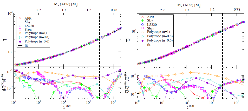
 ,
,
 and
and ![Q¯ = − Q(rot)∕[M 3NS(S∕M N2S )2]](article1242x.gif) ,
,  is the neutron-star mass,
  is
the tidal Love number,
is
the tidal Love number,  is the rotation-induced quadrupole moment, and
  is the magnitude
of the neutron-star spin angular momentum. The neutron-star central density is the parameter varied
along each curve, or equivalently the neutron-star compactness. The top axis shows the neutron star
mass for the APR equation of state, with the vertical dashed line showing
is the magnitude
of the neutron-star spin angular momentum. The neutron-star central density is the parameter varied
along each curve, or equivalently the neutron-star compactness. The top axis shows the neutron star
mass for the APR equation of state, with the vertical dashed line showing  . Bottom:
Relative fractional errors between the fitting curve and the numerical results. Observe that these
relations are essentially independent of the equation of state, with loss of universality at the 1% level.
Image reproduced by permission from [452*], copyright by APS.
. Bottom:
Relative fractional errors between the fitting curve and the numerical results. Observe that these
relations are essentially independent of the equation of state, with loss of universality at the 1% level.
Image reproduced by permission from [452*], copyright by APS.Given the independent measurement of any two members of the I-Love-Q trio, one could carry out a (null) model-independent and equation-of-state-independent test of GR [453*, 452*]. For example, assume that electromagnetic observations of the binary pulsar J0737–3039 have measured the moment of inertia to 10% accuracy [282, 273, 274]. The slow-rotation approximation is perfectly valid for this binary pulsar, due to its relatively long spin period. Assume further that a gravitational-wave observation of a neutron-star–binary inspiral, with individual masses similar to that of the primary in J0737–3039, manages to measure the neutron star tidal Love number to 60% accuracy [453*, 452*]. These observations then lead to an error box in the I-Love plane, which must contain the curve in the left-panel of Figure 5*.
A similar test could be carried out by using data from only binary pulsar observations or only gravitational wave detections. In the case of the latter, one would have to simultaneously measure or constrain the value of the quadrupole moment and the Love number, since the moment of inertia is not measurable with gravitational wave observations. In the case of the former, one would have to extract the moment of inertia and the quadrupole moment, the latter of which will be difficult to measure. Therefore, the combination of electromagnetic and gravitational wave observations would be the ideal way to carry out such tests.
Such a test of GR, of course, is powerful only as long as modified gravity theories predict I-Love-Q
relations that are not degenerated with the general relativistic ones. Yagi and Yunes [453*, 452*] investigated
such a relation in dynamical Chern–Simons gravity to find that such degeneracy is only present in the
limit  . That is, for any finite value of
  , the dynamical Chern–Simons I-Love-Q
relation differs from that of GR, with the distance to the GR expectation increasing for larger
, the dynamical Chern–Simons I-Love-Q
relation differs from that of GR, with the distance to the GR expectation increasing for larger
 . Yagi and Yunes [453*, 452*] predicted that a test similar to the one described above could
constrain dynamical Chern–Simons gravity to roughly
. Yagi and Yunes [453*, 452*] predicted that a test similar to the one described above could
constrain dynamical Chern–Simons gravity to roughly  , where recall that
 .
.
The test described above, of course, only holds provided the I-Love-Q relations are valid, which in turn depends on the assumptions made in deriving them. In particular, Yagi and Yunes [453, 452] assumed that the neutron stars are uniformly and slowly rotating, as well as only slightly tidally deformed by their rotational velocity or companion. These assumptions would not be valid for newly-born neutron stars, which are probably differentially rotating and doing so quickly. However, the gravitational waves emitted by neutron-star inspirals are expected to have binary components that are old and not rapidly spinning by the time they enter the detector sensitivity band [74]. Some short-period, millisecond pulsars may spin at a non-negligible rate, for which the normalized moment of inertia, quadrupole moment and Love number would not be independent of the rotational angular velocity. However, if then the above tests should still be possible, since binary pulsar observations would also automatically determine the rotational angular velocity, for which a unique I-Love-Q relation should exist in GR.
5.4 Tests of the no-hair theorems
Another important class of generic tests of GR are those that concern the no-hair theorems. Since much work has been done on this area, we have decided to separate this topic from the main generic tests section (5.3). In what follows, we describe what these theorems are and the possible tests one could carry out with gravitational-wave observations emitted by black-hole–binary systems.
5.4.1 The no-hair theorems
The no-hair theorems state that the only stationary, vacuum solution to the Einstein equations that is
non-singular outside the event horizon is completely characterized by three quantities: its mass  , its
spin
, its
spin  and its charge
  . This conclusion is arrived at by combining several different theorems. First,
Hawking [223*, 222*] proved that a stationary black hole must have an event horizon with a spherical
topology and that it must be either static or axially symmetric. Israel [243, 244] then proved that the
exterior gravitational field of such static black holes is uniquely determined by
. This conclusion is arrived at by combining several different theorems. First,
Hawking [223*, 222*] proved that a stationary black hole must have an event horizon with a spherical
topology and that it must be either static or axially symmetric. Israel [243, 244] then proved that the
exterior gravitational field of such static black holes is uniquely determined by  and
and  and it must be
given by the Schwarzschild or the Reissner–Nordström metrics. Carter [98] constructed a similar proof
for uncharged, stationary, axially-symmetric black holes, where this time black holes fall into
disjoint families, not deformable into each other and with an exterior gravitational field uniquely
determined by
and it must be
given by the Schwarzschild or the Reissner–Nordström metrics. Carter [98] constructed a similar proof
for uncharged, stationary, axially-symmetric black holes, where this time black holes fall into
disjoint families, not deformable into each other and with an exterior gravitational field uniquely
determined by  and
and  . Robinson [363] and Mazur [306] later proved that such black holes
must be described by either the Kerr or the Kerr–Newman metric. See also [318, 352] for more
details.
. Robinson [363] and Mazur [306] later proved that such black holes
must be described by either the Kerr or the Kerr–Newman metric. See also [318, 352] for more
details.
The no-hair theorems apply under a restrictive set of conditions. First, the theorems only apply in stationary situations. Black-hole horizons can be tidally deformed in dynamical situations, and if so, Hawking’s theorems [223, 222] about spherical horizon topologies do not apply. This then implies that all other theorems described above also do not apply, and thus, dynamical black holes will generically have hair. Second, the theorems only apply in vacuum. Consider, for example, an axially-symmetric black hole in the presence of a non-symmetrical matter distribution outside the event horizon. One might naively think that this would tidally distort the event horizon, leading to a rotating, stationary black hole that is not axisymmetric. However, Hawking and Hartle [226] showed that in such a case the matter distribution torques the black hole forcing it to spin down, thus leading to a non-stationary scenario. If the black hole is non-stationary, then again the no-hair theorems do not apply by the arguments described at the beginning of this paragraph, and thus non-isolated black holes can have hair. Third, the theorems only apply within GR, i.e., through the use of the Einstein equations. Therefore, it is plausible that black holes in modified gravity theories or in GR with singularities outside any event horizons (naked singularities) will have hair.
The no-hair theorems imply that the exterior gravitational field of isolated, stationary, uncharged and
vacuum black holes (in GR and provided the spacetime is regular outside all event horizons) can be written
as an infinite sum of mass and current multipole moments, where only two of them are independent: the
mass monopole moment  and the current dipole moment
  . One can extend these relations to
include charge, but astrophysical black holes are expected to be essentially neutral due to charge accretion.
If the no-hair theorems hold, all other multipole moments can be determined from [195, 194, 213]
. One can extend these relations to
include charge, but astrophysical black holes are expected to be essentially neutral due to charge accretion.
If the no-hair theorems hold, all other multipole moments can be determined from [195, 194, 213]

 and
and  are the
  th mass and current multipole moments. Even if the black-hole progenitor
was not stationary or axisymmetric, the no-hair theorems guarantee that any excess multipole moments will
be shed-off during gravitational collapse [356, 357]. Eventually, after the black hole has settled down and
reached an equilibrium configuration, it will be described purely in terms of
th mass and current multipole moments. Even if the black-hole progenitor
was not stationary or axisymmetric, the no-hair theorems guarantee that any excess multipole moments will
be shed-off during gravitational collapse [356, 357]. Eventually, after the black hole has settled down and
reached an equilibrium configuration, it will be described purely in terms of  and
and
 , where
  is the Kerr spin parameter.
An astrophysical observation of a hairy black hole would not imply that the no-hair theorems are wrong, but rather that one of the assumptions made in deriving these theorems is not appropriate to describe nature. As described above, the three main assumptions are stationarity, vacuum and that GR and the regularity condition hold. Astrophysical black holes will generically be hairy due to a violation of the first two assumptions, since they will neither be perfectly stationary, nor exist in a perfect vacuum. Astrophysical black holes will always suffer small perturbations by other stars, electromagnetic fields, other forms of matter, like dust, plasma or dark matter, etc, which will induce non-zero deviations from Eq. (219*) and thus evade the no-hair theorems. However, in all cases of interest such perturbations are expected to be too small to be observable, which is why one argues that even astrophysical black holes should obey the no-hair theorems if GR holds. Put another way, an observation of the violation of the no-hair theorems would be more likely to indicate a failure of GR in the strong-field, than an unreasonably large amount of astrophysical hair.
Tests of the no-hair theorems come in two flavors: through electromagnetic observations [250, 251, 253, 254] and through gravitational wave observations [370*, 371*, 112*, 196*, 44*, 50, 289, 390*, 471, 422*, 421*, 184*, 423*, 364]. The former rely on radiation emitted by accelerating particles in an accretion disk around black holes. However, such tests are not clean as they require the modeling of complicated astrophysics, with matter and electromagnetic fields. Gravitational wave tests are clean in that respect, but unlike electromagnetic tests, they cannot be carried out yet due to lack of data. Other electromagnetic tests of the no-hair theorems exist, for example through the observation of close stellar orbits around Sgr A* [312, 313, 373] and pulsar–black-hole binaries [431], but these cannot yet probe the near-horizon, strong-field regime, since electromagnetic observations cannot yet resolve horizon scales. See [359] for reviews on this topic.
5.4.2 Extreme mass-ratio tests of the no-hair theorem
Gravitational wave tests of the no-hair theorems require the detection of either extreme mass-ratio inspirals or the ringdown of comparable-mass black-hole mergers with future space-borne gravitational-wave detectors [25, 24]. Extreme mass-ratio inspirals consist of a stellar-mass compact object spiraling into a supermassive black hole in a generic orbit within astronomical units from the event horizon of the supermassive object [23]. These events outlive the observation time of future detectors, emitting millions of gravitational wave cycles, with the stellar-mass compact object essentially acting as a tracer of the supermassive black hole spacetime [397]. Ringdown gravitational waves are always emitted after black holes merge and the remnant settles down into its final configuration. During the ringdown, the highly-distorted remnant radiates all excess degrees of freedom and this radiation carries a signature of whether the no-hair theorems hold in its quasi-normal mode spectrum (see, e.g., [68*] for a recent review).
Both electromagnetic and gravitational wave tests need a metric with which to model accretion disks,
quasi-periodic oscillations, or extreme mass-ratio inspirals. One can classify these metrics as direct or
generic, paralleling the discussion in Section 5.2. Direct metrics are exact solutions to a specific set of field
equations, with which one can derive observables. Examples of such metrics are the Manko–Novikov
metric [302] and the slowly-spinning black-hole metric in dynamical Chern–Simons gravity [466*]. When
computing observables with these metrics, one usually assumes that all radiative and dynamical process
(e.g., the radiation-reaction force) are as predicted in GR. Generic metrics are those that parametrically
modify the Kerr spacetime, such that for certain parameter choices one recovers identically the
Kerr metric, while for others, one has a deformation of Kerr. Generic metrics can be further
classified into two subclasses, Ricci-flat versus non-Ricci-flat, depending on whether they satisfy
 .
.
Let us first consider direct metric tests of the no-hair theorem. The most studied direct metric is the Manko–Novikov one, which although an exact, stationary and axisymmetric solution to the vacuum Einstein equations, does not represent a black hole, as the event horizon is broken along the equator by a ring singularity [302]. Just like the Kerr metric, the Manko–Novikov metric possesses an ergoregion, but unlike the former, it also possesses regions of closed time-like curves that overlap the ergoregion. Nonetheless, an appealing property of this metric is that it deviates continuously from the Kerr metric through certain parameters that characterize the higher multiple moments of the solution.
The first geodesic study of Manko–Novikov spacetimes was carried out by Gair et al. [182*]. They found that there are two ring-like regions of bound orbits: an outer one where orbits look regular and integrable, as there exist four isolating integrals of the motion; and an inner one where orbits are chaotic and thus ergodic. Gair et al. [182*] suggested that orbits that transition from the integrable to the chaotic region would leave a clear observable signature in the frequency spectrum of the emitted gravitational waves. However, they also noted that chaotic regions exist only very close to the central body and are probably not astrophysically accessible. The study of Gair et al. [182] was recently confirmed and followed up by Contopoulos et al. [116]. They studied a wide range of geodesics and found that, in addition to an inner chaotic region and an outer regular region, there are also certain Birkhoff islands of stability. When an extreme mass-ratio inspiral traverses such a region, the ratio of resonant fundamental frequencies would remain constant in time, instead of increasing monotonically. Such a feature would impact the gravitational waves emitted by such a system, and it would signal that the orbit equations are non-integrable and the central object is not a Kerr black hole.
The study of chaotic motion in geodesics of non-Kerr spacetimes is by no means new. Chaos has also been found in geodesics of Zipoy–Voorhees–Weyl and Curzon spacetimes with multiple singularities [391, 392] and in general for Zipoy–Voorhees spacetimes in [296], of perturbed Schwarzschild spacetimes [287], of Schwarzschild spacetimes with a dipolar halo [286, 288, 209] of Erez–Rosen spacetimes [210], and of deformed generalizations of the Tomimatsy–Sato spacetime [154]. One might worry that such chaotic orbits will depend on the particular spacetime considered, but recently Apostolatos et al. [31*] and Lukes–Gerakopoulos et al. [297*] have argued that the Birkhoff islands of stability are a general feature. Although the Kolmogorov, Arnold, and Moser theorem [270, 35, 321] states that phase orbit tori of an integrable system are only deformed if the Hamiltonian is perturbed, the Poincare–Birkhoff theorem [292] states that resonant tori of integrable systems actually disintegrate, leaving behind a chain of Birkhoff islands. These islands are only characterized by the ratio of winding frequencies that equals a rational number, and thus, they constitute a distinct and generic feature of non-integrable systems [31, 297]. Given an extreme mass-ratio gravitational-wave detection, one can monitor the ratio of fundamental frequencies and search for plateaus in their evolution, which would signal non-integrability. Of course, whether detectors can resolve such plateaus depends on the initial conditions of the orbits and the physical system under consideration (these determine the thickness of the islands), as well as the mass ratio (this determines the radiation-reaction timescale) and the distance and mass of the central black hole (this determines the SNR).
Another example of a direct metric test of the no-hair theorem is through the use of the slowly-rotating dynamical Chern–Simons black hole metric [466]. Unlike the Manko–Novikov metric, the dynamical Chern–Simons one does represent a black hole, i.e., it possesses an event horizon, but it evades the no-hair theorems because it is not a solution to the Einstein equations. Sopuerta and Yunes [390] carried out the first extreme mass-ratio inspiral analysis when the background supermassive black hole object is taken to be such a Chern–Simons black hole. They used a semi-relativistic model [368] to evolve extreme mass-ratio inspirals and found that the leading-order modification comes from a modification to the geodesic trajectories, induced by the non-Kerr modifications of the background. Because the latter correspond to a strong-field modification to GR, modifications in the trajectories are most prominent for zoom-whirl orbits, as the small compact object zooms around the supermassive black hole in a region of unstable orbits, close to the event horizon. These modifications were then found to propagate into the gravitational waves emitted, leading to a dephasing that could be observed or ruled out with future gravitational-wave observations to roughly the horizon scale of the supermassive black hole, as has been recently confirmed by Canizares et al. [93]. However, these studies may be underestimates, given that they treat the black hole background in dynamical Chern–Simons gravity only to first-order in spin.
A final example of a direct metric test of the no-hair theorems is to consider black holes that are not in vacuum. Barausse et al. [52] studied extreme–mass-ratio inspirals in a Kerr–black-hole background that is perturbed by a self-gravitating, homogeneous torus that is compact, massive and close to the Kerr black hole. They found that the presence of this torus impacts the gravitational waves emitted during such inspirals, but only weakly, making it difficult to distinguish the presence of matter. Yunes et al. [462] and Kocsis et al. [267] carried out a similar study, where this time they considered a small compact object inspiraling completely within a geometrically thin, radiation-pressure dominated accretion disk. They found that disk-induced migration can modify the radiation-reaction force sufficiently so as to leave observable signatures in the waveform, provided the accretion disk is sufficiently dense in the radiation-dominated regime and a gap opens up. However, these tests of the no-hair theorem will be rather difficult as most extreme–mass-ratio inspirals are not expected to be in an accretion disk.
Let us now consider generic metric tests of the no-hair theorem. Generic Ricci-flat deformed metrics will
lead to Laplace-type equations for the deformation functions in the far-field since they must satisfy
 to linear order in the perturbations. The solution to such an equation can be expanded in
a sum of mass and current multipole moments, when expressed in asymptotically Cartesian
and mass-centered coordinates [407]. These multipoles can be expressed via [112*, 422*, 421*]
to linear order in the perturbations. The solution to such an equation can be expanded in
a sum of mass and current multipole moments, when expressed in asymptotically Cartesian
and mass-centered coordinates [407]. These multipoles can be expressed via [112*, 422*, 421*]

 and
and  are mass and current multipole deformations. Ryan [370, 371] showed that the
measurement of three or more multipole moments would allow for a test of the no-hair theorem. Generic
non-Ricci flat metrics, on the other hand, will not necessarily lead to Laplace-type equations for the
deformation functions in the far field, and thus, the far-field solution and Eq. (220*) will depend on a sum of
are mass and current multipole deformations. Ryan [370, 371] showed that the
measurement of three or more multipole moments would allow for a test of the no-hair theorem. Generic
non-Ricci flat metrics, on the other hand, will not necessarily lead to Laplace-type equations for the
deformation functions in the far field, and thus, the far-field solution and Eq. (220*) will depend on a sum of
 and
and  multipole moments.
The first attempt to construct a generic, Ricci-flat metric was by Collins and Hughes [112*]: the bumpy black-hole metric. In this approach, the metric is assumed to be of the form
where
 is a bookkeeping parameter that enforces that
  is a perturbation of the Kerr
background. This metric is then required to satisfy the Einstein equations linearized in
is a perturbation of the Kerr
background. This metric is then required to satisfy the Einstein equations linearized in  , which then
leads to differential equations for the metric deformation. Collins and Hughes [112*] assumed a non-spinning,
stationary spacetime, and thus
, which then
leads to differential equations for the metric deformation. Collins and Hughes [112*] assumed a non-spinning,
stationary spacetime, and thus  only possessed two degrees of freedom, both of which were
functions of radius only:
only possessed two degrees of freedom, both of which were
functions of radius only:  , which must be a harmonic function and which changes the
Newtonian part of the gravitational field at spatial infinity; and
, which must be a harmonic function and which changes the
Newtonian part of the gravitational field at spatial infinity; and  which is completely
determined through the linearized Einstein equations once
which is completely
determined through the linearized Einstein equations once  is specified. One then has the
freedom to choose how to prescribe
is specified. One then has the
freedom to choose how to prescribe  and Collins and Hughes investigate [112] two choices
that correspond physically to point-like and ring-like naked singularities, thus violating cosmic
censorship [347]. Vigeland and Hughes [422] and Vigeland [421] then extend this analysis to stationary,
axisymmetric spacetimes via the Newman–Janis method [327*, 151*], showing how such metric
deformations modify Eq. (220*), and computing how these bumps imprint themselves onto the
orbital frequencies and thus the gravitational waves emitted during an extreme–mass-ratio
inspiral.
and Collins and Hughes investigate [112] two choices
that correspond physically to point-like and ring-like naked singularities, thus violating cosmic
censorship [347]. Vigeland and Hughes [422] and Vigeland [421] then extend this analysis to stationary,
axisymmetric spacetimes via the Newman–Janis method [327*, 151*], showing how such metric
deformations modify Eq. (220*), and computing how these bumps imprint themselves onto the
orbital frequencies and thus the gravitational waves emitted during an extreme–mass-ratio
inspiral.
That the bumps represent unphysical matter should not be a surprise, since by the no-hair theorems, if the bumps are to satisfy the vacuum Einstein equations they must either break stationarity or violate the regularity condition. Naked singularities are an example of the latter. A Lorentz-violating massive field coupled to the Einstein tensor is another example [155]. Gravitational wave tests with bumpy black holes must then be understood as null tests: one assumes the default hypothesis that GR is correct and then sets out to test whether the data rejects or fails to reject this hypothesis (a null hypothesis can never be proven). Unfortunately, however, bumpy black hole metrics cannot parameterize spacetimes in modified gravity theories that lead to corrections in the field equations that are not proportional to the Ricci tensor, such as for example in dynamical Chern–Simons or in Einstein-Dilaton-Gauss–Bonnet modified gravity.
Other bumpy black hole metrics have also been recently proposed. Glampedakis and Babak [196*]
proposed a different type of stationary and axisymmetric bumpy black hole through the Hartle–Thorne
metric [218], with modifications to the quadrupole moment. They then constructed a “kludge” extreme
mass-ratio inspiral waveform and estimated how well the quadrupole deformation could be measured [44*].
However, this metric is valid only when the supermassive black hole is slowly-rotating, as it derives from the
Hartle–Thorne ansatz. Recently, Johansen and Psaltis [252*] proposed yet another metric to represent
bumpy stationary and spherically-symmetric spacetimes. This metric introduces one new degree of
freedom, which is a function of radius only and assumed to be a series in  . Johansen and
Psaltis then rotated this metric via the Newman–Janis method [327, 151] to obtain a new
bumpy metric for axially-symmetric spacetimes. However, such a metric possesses a naked ring
singularity on the equator, and naked singularities on the poles. As before, none of these bumpy
metrics can be mapped to known modified gravity black hole solutions, in the Glampedakis
and Babak case [196] because the Einstein equations are assumed to hold to leading order in
the spin, while in the Johansen and Psaltis case [252] because a single degree of freedom is
not sufficient to model the three degrees of freedom contained in stationary and axisymmetric
spacetimes [401, 423*].
. Johansen and
Psaltis then rotated this metric via the Newman–Janis method [327, 151] to obtain a new
bumpy metric for axially-symmetric spacetimes. However, such a metric possesses a naked ring
singularity on the equator, and naked singularities on the poles. As before, none of these bumpy
metrics can be mapped to known modified gravity black hole solutions, in the Glampedakis
and Babak case [196] because the Einstein equations are assumed to hold to leading order in
the spin, while in the Johansen and Psaltis case [252] because a single degree of freedom is
not sufficient to model the three degrees of freedom contained in stationary and axisymmetric
spacetimes [401, 423*].
The only generic non-Ricci-flat bumpy black-hole metric so far is that of Vigeland, Yunes and
Stein [423*]. They allowed generic deformations in the metric tensor, only requiring that the new metric
perturbatively retained the Killing symmetries of the Kerr spacetime: the existence of two Killing
vectors associated with stationarity and axisymmetry, as well as the perturbative existence
of a Killing tensor (and thus a Carter-like constant), at least to leading order in the metric
deformation. Such requirements imply that the geodesic equations in this new background are
fully integrable, at least perturbatively in the metric deformation, which then allows one to
solve for the orbital motion of extreme–mass-ratio inspirals by adapting previously existing
tools. Brink [83, 84, 85, 86, 87] studied the existence of such a second-order Killing tensor in
generic, vacuum, stationary and axisymmetric spacetimes in Einstein’s theory and found that
these are difficult to construct exactly. By relaxing this exact requirement, Vigeland, Yunes and
Stein [423] found that the existence of a perturbative Killing tensor poses simple differential
conditions on the metric perturbation that can be analytically solved. Moreover, they also showed
how this new bumpy metric can reproduce all known modified gravity black hole solutions in
the appropriate limits, provided these have an at least approximate Killing tensor; thus, these
metrics are still vacuum solutions even though  , since they satisfy a set of modified field
equations. Although unclear at this junction, it seems that the imposition that the spacetime retains
the Kerr Killing symmetries leads to a bumpy metric that is well-behaved everywhere outside
the event horizon (no singularities, no closed-time-like curves, no loss of Lorentz signature).
Recently, Gair and Yunes [184] studied how the geodesic equations are modified for a test-particle
in a generic orbit in such a spacetime and showed that the bumps are indeed encoded in the
orbital motion, and thus, in the gravitational waves emitted during an extreme–mass-ratio
inspiral.
, since they satisfy a set of modified field
equations. Although unclear at this junction, it seems that the imposition that the spacetime retains
the Kerr Killing symmetries leads to a bumpy metric that is well-behaved everywhere outside
the event horizon (no singularities, no closed-time-like curves, no loss of Lorentz signature).
Recently, Gair and Yunes [184] studied how the geodesic equations are modified for a test-particle
in a generic orbit in such a spacetime and showed that the bumps are indeed encoded in the
orbital motion, and thus, in the gravitational waves emitted during an extreme–mass-ratio
inspiral.
One might be concerned that such no-hair tests of GR cannot constrain modified gravity theories, because Kerr black holes can also be solutions in the latter [360]. This is indeed true provided the modified field equations depend only on the Ricci tensor or scalar. In Einstein-Dilaton-Gauss–Bonnet or dynamical Chern–Simons gravity, the modified field equations depend on the Riemann tensor, and thus, Ricci-flat metric need not solve these modified set [473]. Moreover, just because the metric background is identically Kerr does not imply that inspiral gravitational waves will be identical to those predicted in GR. All studies carried out to date, be it direct metric tests or generic metric tests, assume that the only quantity that is modified is the metric tensor, or equivalently, the Hamiltonian or binding energy. Inspiral motion, of course, does not depend just on this quantity, but also on the radiation-reaction force that pushes the small object from geodesic to geodesic. Moreover, the gravitational waves generated during such an inspiral depend on the field equations of the theory considered. Therefore, all metric tests discussed above should be considered as partial tests. In general, strong-field modified gravity theories will modify the Hamiltonian, the radiation-reaction force and the wave generation.
5.4.3 Ringdown tests of the no-hair theorem
Let us now consider tests of the no-hair theorems with gravitational waves emitted by comparable-mass binaries during the ringdown phase. Gravitational waves emitted during ringdown can be described by a superposition of exponentially-damped sinusoids [69*]:
where
 is the distance from the source to the detector, the asterisk stands for complex conjugation, the
real mode amplitudes
is the distance from the source to the detector, the asterisk stands for complex conjugation, the
real mode amplitudes  and
and  and the real phases
  and
and  depend on the initial
conditions,
depend on the initial
conditions,  are spheroidal functions evaluated at the complex quasinormal ringdown frequencies
 , and the real physical frequency
  and the real damping times
  are
both functions of the mass
are
both functions of the mass  and the Kerr spin parameter
  only, provided the no-hair theorems hold.
These frequencies and damping times can be computed numerically or semi-analytically, given a particular
black-hole metric (see [68] for a recent review). The Fourier transform of a given
only, provided the no-hair theorems hold.
These frequencies and damping times can be computed numerically or semi-analytically, given a particular
black-hole metric (see [68] for a recent review). The Fourier transform of a given  mode
is [69*]
mode
is [69*]
where we have defined  as well as the Lorentzian functions

Tests of the no-hair theorems through the observation of black-hole ringdown date back to
Detweiler [146], and it was recently worked out in detail by Dreyer et al. [152*]. Let us first imagine that a
single complex mode is detected  and one measures separately its real and imaginary
parts. Of course, from such a measurement, one cannot extract the measured harmonic triplet
and one measures separately its real and imaginary
parts. Of course, from such a measurement, one cannot extract the measured harmonic triplet
 , but instead one only measures the complex frequency
  . This information is not
sufficient to extract the mass and spin angular momentum of the black hole because different
quintuplets
. This information is not
sufficient to extract the mass and spin angular momentum of the black hole because different
quintuplets  can lead to the same complex frequency
  . The best way
to think of this is graphically: a given observation of
. The best way
to think of this is graphically: a given observation of  traces a line in the complex
 plane; a given
  triplet defines a complex frequency
  that also traces a curve in the complex
  plane; each intersection of the measured line
 with
with  defines a possible doublet
  ; since different
  triplets lead to
different
triplets lead to
different  curves and thus different intersections, one ends up with a set of doublets
  ,
out of which only one represents the correct black-hole parameters. We thus conclude that a
single mode observation of ringdown gravitational waves is not sufficient to test the no-hair
theorem [152*, 69*].
,
out of which only one represents the correct black-hole parameters. We thus conclude that a
single mode observation of ringdown gravitational waves is not sufficient to test the no-hair
theorem [152*, 69*].
Let us then imagine that one has detected two complex modes,  and
and  . Each
detection leads to a separate line
. Each
detection leads to a separate line  and
and  in the complex plane. As before, each
 triplet leads to separate curves
  which will intersect with both
  and
and
 in the complex plane. Each intersection between
  and
and  leads to a
set of doublets
leads to a
set of doublets  , while each intersection between
  and
and  leads to another
set of doublets
leads to another
set of doublets  . However, if the no-hair theorems hold sets
  and
and  must have at
least one element in common. Therefore, a two-mode detection allows for tests of the no-hair
theorem [152, 69*]. However, when dealing with a quasi-circular black-hole–binary inspiral within GR one
knows that the dominant mode is
must have at
least one element in common. Therefore, a two-mode detection allows for tests of the no-hair
theorem [152, 69*]. However, when dealing with a quasi-circular black-hole–binary inspiral within GR one
knows that the dominant mode is  . In such a case, the observation of this complex
mode by itself allows one to extract the mass and spin angular momentum of the black hole.
Then, the detection of the real frequency in an additional mode can be used to test the no-hair
theorem [69*, 65*].
. In such a case, the observation of this complex
mode by itself allows one to extract the mass and spin angular momentum of the black hole.
Then, the detection of the real frequency in an additional mode can be used to test the no-hair
theorem [69*, 65*].
Although the logic behind these tests is clear, one must study them carefully to determine whether all
systematic and statistical errors are sufficiently under control so that they are feasible. Berti et al. [69*, 65*]
investigated such tests carefully through a frequentist approach. First, they found that a matched-filtering
type analysis with two-mode ringdown templates would increase the volume of the template manifold by
roughly three orders of magnitude. A better strategy then is perhaps to carry out a Bayesian analysis,
like that of Gossan et al. [256, 201]; through such a study one can determine whether a given
detection is consistent with a two-mode or a one-mode hypothesis. Berti et al. [69, 65] also
calculated that a SNR of  would be sufficient to detect the presence of two modes in the
ringdown signal and to resolve their frequencies, so that no-hair tests would be possible. Strong
signals are necessary because one must be able to distinguish at least two modes in the signal.
Unfortunately, however, whether the ringdown leads to such strong SNRs and whether the sub-dominant
ringdown modes are of a sufficiently large amplitude depends on a plethora of conditions: the
location of the source in the sky, the mass of the final black hole, which depends on the rest mass
fraction that is converted into ringdown gravitational waves (the ringdown efficiency), the mass
ratio of the progenitor, the magnitude and direction of the spin angular momentum of the final
remnant and probably also of the progenitor and the initial conditions that lead to ringdown.
Thus, although such tests are possible, one would have to be quite fortunate to detect a signal
with the right properties so that a two-mode extraction and a test of the no-hair theorems is
feasible.
would be sufficient to detect the presence of two modes in the
ringdown signal and to resolve their frequencies, so that no-hair tests would be possible. Strong
signals are necessary because one must be able to distinguish at least two modes in the signal.
Unfortunately, however, whether the ringdown leads to such strong SNRs and whether the sub-dominant
ringdown modes are of a sufficiently large amplitude depends on a plethora of conditions: the
location of the source in the sky, the mass of the final black hole, which depends on the rest mass
fraction that is converted into ringdown gravitational waves (the ringdown efficiency), the mass
ratio of the progenitor, the magnitude and direction of the spin angular momentum of the final
remnant and probably also of the progenitor and the initial conditions that lead to ringdown.
Thus, although such tests are possible, one would have to be quite fortunate to detect a signal
with the right properties so that a two-mode extraction and a test of the no-hair theorems is
feasible.
5.4.4 The hairy search for exotica
Another way to test GR is to modify the matter sector of the theory through the introduction of matter corrections to the Einstein–Hilbert action that violate the assumptions made in the no-hair theorems. More precisely, one can study whether gravitational waves emitted by binaries composed of strange stars, like quark stars, or horizonless objects, such as boson stars or gravastars, are different from waves emitted by more traditional neutron-star or black-hole binaries. In what follows, we will describe such hairy tests of the existence of compact exotica.
Boson stars are a classic example of a compact object that is essentially indistinguishable from a black hole in the weak field, but which differs drastically from one in the strong field due to its lack of an event horizon. A boson star is a coherent scalar-field configuration supported against gravitational collapse by its self-interaction. One can construct several Lagrangian densities that would allow for the existence of such an object, including mini-boson stars [178, 179], axially-symmetric solitons [372], and nonsolitonic stars supported by a non-canonical scalar potential energy [113]. Boson stars are well-motivated from fundamental theory, since they are the gravitationally-coupled limit of q-balls [108, 276], a coherent scalar condensate that can be described classically as a non-topological soliton and that arises unavoidably in viable supersymmetric extensions of the standard model [275]. In all studies carried out to date, boson stars have been studied within GR, but they are also allowed in scalar-tensor theories [46].
At this junction, one should point out that the choice of a boson star is by no means special; the key point here is to select a straw-man to determine whether gravitational waves emitted during the coalescence of compact binaries are sensitive to the presence of an event horizon or the evasion of the no-hair theorems induced by a non-vacuum spacetime. Of course, depending on the specific model chosen, it is possible that the exotic object will be unstable to evolution or even to its own rotation. For example, in the case of an extreme mass-ratio inspiral, one could imagine that as the small compact object enters the boson star’s surface, it will accrete the scalar field, forcing the boson star to collapse into a black hole. Alternatively, one can imagine that as two supermassive boson stars merge, the remnant might collapse into a black hole, emitting the usual GR quasinormal modes. What is worse, even when such objects are in isolation, they are unstable under small perturbations if their angular momentum is large, possibly leading to gravitational collapse into a black hole or possibly a scalar explosion [95, 96]. Since most astrophysical black hole candidates are believed to have high spins, such instabilities somewhat limit the interest of horizonless objects. Even then, however, the existence of slowly spinning or non spinning horizonless compact objects cannot be currently ruled out by observation.
Boson stars evade the no-hair theorems within GR because they are not vacuum spacetimes, and thus, their metric and quasinormal mode spectrum cannot be described by just their mass and spin angular momentum; one also requires other quantities intrinsic to the scalar-field energy momentum tensor, scalar hair. Therefore, as before, two types of gravitational wave tests for scalar hair have been proposed: extreme–mass-ratio inspiral tests and ringdown tests. As for the former, several studies have been carried out that considered a supermassive boson star background. Kesden et al. [263*] showed that stable circular orbits exist both outside and inside of the surface of the boson star, provided the small compact object interacts with the background only gravitationally. This is because the effective potential for geodesic motion in such a boson-star background lacks the Schwarzschild-like singular behavior at small radius, instead turning over and allowing for a new minimum. Gravitational waves emitted in such a system would then stably continue beyond what one would expect if the background had been a supermassive black hole; in the latter case the small compact object would simply disappear into the horizon. Kesden et al. [263] found that orbits inside the boson star exhibit strong precession, exciting high frequency harmonics in the waveform, and thus allowing one to easily distinguish between such boson stars from black-hole backgrounds.
Just as the inspiral phase is modified by the presence of a boson star, the merger phase is also greatly altered, but this must be treated fully numerically. A few studies have found that the merger of boson stars leads to a spinning bar configuration that either fragments or collapses into a Kerr black hole [339, 338]. Of course, the gravitational waves emitted during such a merger will be drastically different from those produced when black holes merge. Unfortunately, the complexity of such simulations makes predictions difficult for any one given example, and the generalization to other more complicated scenarios, such as theories with modified field equations, is currently not feasible.
Recently, Pani et al. [340*, 341*] revisited this problem, but instead of considering a supermassive boson star, they considered a gravastar. This object consists of a Schwarzschild exterior and a de Sitter interior, separated by an infinitely thin shell with finite tension [307, 100]. Pani et al. [341*] calculated the gravitational waves emitted by a stellar-mass compact object in a quasi-circular orbit around such a gravastar background. In addition to considering a different background, Pani et al. used a radiative-adiabatic waveform generation model to describe the gravitational waves [351, 238, 239, 458, 456, 459], instead of the kludge scheme used by Kesden et al. [49, 44, 456]. Pani el al. [341] concluded that the waves emitted during such inspirals are sufficiently different that they could be used to discern between a Kerr black hole and a gravastar.
On the ringdown side of no-hair tests, several studies have been carried out. Berti and Cardoso [66] calculated the quasi-normal mode spectrum of boson stars. Chirenti and Rezzolla [105] studied the non-radial, axial perturbations of gravastars, and Pani et al. [340] the non-radial, axial and polar oscillations of gravastars. Medved et al. [309, 310] considered the quasinormal ringdown spectrum of skyrmion black holes [386]. In all cases, it was found that the quasi-normal mode spectrum of such objects could be used to discern between them and Kerr black holes. Of course, such tests still require the detection of ringdown gravitational waves with the right properties, such that more than one mode can be discerned and extracted from the signal (see Section 5.4.3).
 |
 |
 |
Living Rev. Relativity, 16 (2013), 9, doi:10.12942/lrr-2013-9, URL (accessed <date>): http://www.livingreviews.org/lrr-2013-9.
 This work is licensed under a Creative Commons License.
© The author(s), except where otherwise noted.
This work is licensed under a Creative Commons License.
© The author(s), except where otherwise noted.