 -decoupling
limit of bi-gravity
-decoupling
limit of bi-gravity
 )
)10 Massive Gravity Field Theory
10.1 Vainshtein mechanism
As seen earlier, in four dimensions a massless spin-2 field has five degrees of freedom, and there is no special PM case of gravity where the helicity-0 mode is unphysical while the graviton remains massive (or at least there is to date no known such theory). The helicity-0 mode couples to matter already at the linear level and this additional coupling leads to a extra force which is at the origin of the vDVZ discontinuity see in Section 2.2.3. In this section, we shall see how the non-linearities of the helicity-0 mode is responsible for a Vainshtein mechanism that screens the effect of this field in the vicinity of matter.
Since the Vainshtein mechanism relies strongly on non-linearities, this makes explicit solutions very hard to find. In most of the cases where the Vainshtein mechanism has been shown to work successfully, one assumes a static and spherically symmetric background source. Already in that case the existence of consistent solutions which extrapolate from a well-behaved asymptotic behavior at infinity to a screened solution close to the source are difficult to obtain numerically [121] and were only recently unveiled [37*, 39*] in the case of non-linear Fierz–Pauli gravity.
This review on massive gravity cannot do justice to all the ongoing work dedicated to the study of the Vainshtein mechanism (also sometimes called ‘kinetic chameleon’ as it relies on the kinetic interactions for the helicity-0 mode). In what follows, we will give the general idea behind the Vainshtein mechanism starting from the decoupling limit of massive gravity and then show explicit solutions in the decoupling limit for static and spherically symmetric sources. Such an analysis is relevant for observational tests in the solar system as well as for other astrophysical tests (such as binary pulsar timing), which we shall explore in Section 11. We refer to the following review on the Vainshtein mechanism for further details, [35] as well as to the following work [160*, 38*, 99*, 332, 36, 244, 40, 338, 321, 440*, 316, 53, 376, 366, 407*]. Recently, it was also shown that the Vainshtein mechanism works for bi-gravity, see Ref. [34].
We focus the rest of this section to the case of four space-time dimensions, although many of the results presented in what follows are well understood in arbitrary dimensions.
10.1.1 Effective coupling to matter
As already mentioned, the key ingredient behind the Vainshtein mechanism is the importance of
interactions for the helicity-0 mode which we denote as  . From the decoupling limit analysis
performed for massive gravity (see (8.52*)) and bi-gravity (see (8.78*)), we see that in some
limit the helicity-0 mode
. From the decoupling limit analysis
performed for massive gravity (see (8.52*)) and bi-gravity (see (8.78*)), we see that in some
limit the helicity-0 mode  behaves as a scalar field, which enjoys a special global symmetry

These types of interactions are very similar to the Galileon-type of interactions introduced by Nicolis, Rattazzi and Trincherini in Ref. [412*] as a generalization of the decoupling limit of DGP. For simplicity we shall focus most of the discussion on the Vainshtein mechanism with Galileons as a special example, and then mention in Section 10.1.3 peculiarities that arise in the special case of massive gravity (see for instance Refs. [58*, 57*]).
We thus start with a cubic Galileon theory
where
 is the trace of the stress-energy tensor of external sources, and
  is the strong coupling
scale of the theory. As seen earlier, in the case of massive gravity,
is the strong coupling
scale of the theory. As seen earlier, in the case of massive gravity,  . This is actually
precisely the way the helicity-0 mode enters in the decoupling limit of DGP [389] as seen in
Section 4.2. It is in that very context that the Vainshtein mechanism was first shown to work
explicitly [165].
. This is actually
precisely the way the helicity-0 mode enters in the decoupling limit of DGP [389] as seen in
Section 4.2. It is in that very context that the Vainshtein mechanism was first shown to work
explicitly [165].
The essence of the Vainshtein mechanism is that close to a source, the Galileon interactions dominate
over the linear piece. We make use of this fact by splitting the source into a background contribution  and a perturbation
  . The background source
  leads to a background profile
  for the field, and
the response to the fluctuation
for the field, and
the response to the fluctuation  on top of this background is given by
  , so that the total field is
expressed as
, so that the total field is
expressed as

 represents a static point-like
source, then sufficiently close to the source), the non-linearities dominate and symbolically
represents a static point-like
source, then sufficiently close to the source), the non-linearities dominate and symbolically
 .
.
We now follow the perturbations in the action (10.2*) and notice that the background configuration  leads to a modified effective metric for the perturbations,

 where the tensor
 is the same as that defined for massive gravity in (8.29*) or in (8.34*), so
symbolically
is the same as that defined for massive gravity in (8.29*) or in (8.34*), so
symbolically  is of the form
  . One can generalize the initial action (10.2*) to arbitrary set
of Galileon interactions
with again
. One can generalize the initial action (10.2*) to arbitrary set
of Galileon interactions
with again ![4 ℒ = π∑ --cn+1-ℒ [Π], (10.6 ) Λ3 (n− 1) n n=1](article1864x.gif)
 and where the scalars
  have been defined in (6.10*) – (6.13*). The effective
metric would then be of the form
where all the tensors
have been defined in (6.10*) – (6.13*). The effective
metric would then be of the form
where all the tensors 
 are defined in (8.28*) – (8.32*). Notice that
  identically. For
sufficiently large sources, the components of
identically. For
sufficiently large sources, the components of  are large, symbolically,
  for
for
 .
.
Canonically normalizing the fluctuations in (10.4*), we have symbolically,
assuming
 , which is not generally the case. Nevertheless, this symbolic scaling is sufficient to
get the essence of the idea. For a more explicit canonical normalization in specific configurations
see Ref. [412*]. As nicely explained in that reference, if
, which is not generally the case. Nevertheless, this symbolic scaling is sufficient to
get the essence of the idea. For a more explicit canonical normalization in specific configurations
see Ref. [412*]. As nicely explained in that reference, if  is conformally flat, one should
not only scale the field
is conformally flat, one should
not only scale the field  but also the space-like coordinates
  so at to obtain
a standard canonically normalized field in the new system,
so at to obtain
a standard canonically normalized field in the new system,  . For now we
stick to the simple normalization (10.8*) as it is sufficient to see the essence of the Vainshtein
mechanism. In terms of the canonically normalized field
. For now we
stick to the simple normalization (10.8*) as it is sufficient to see the essence of the Vainshtein
mechanism. In terms of the canonically normalized field  , the perturbed action (10.4*) is then
which means that the coupling of the fluctuations to matter is medium dependent and can arise at a scale
very different from the Planck scale. In particular, for a large background configuration,
, the perturbed action (10.4*) is then
which means that the coupling of the fluctuations to matter is medium dependent and can arise at a scale
very different from the Planck scale. In particular, for a large background configuration, 
 and
and
 , so the effective coupling scale to external matter is
and the coupling to matter is thus very suppressed. In massive gravity
, so the effective coupling scale to external matter is
and the coupling to matter is thus very suppressed. In massive gravity 
 is related to the graviton mass,
 , and so the effective coupling scale
  as
as  , which shows how the helicity-0
mode characterized by
, which shows how the helicity-0
mode characterized by  decouples in the massless limit.
We now first review how the Vainshtein mechanism works more explicitly in a static and spherically symmetric configuration before applying it to other systems. Note that the Vainshtein mechanism relies on irrelevant operators. In a standard EFT this cannot be performed without going beyond the regime of validity of the EFT. In the context of Galileons and other very specific derivative theories, one can reorganize the EFT so that the operators considered can be large and yet remain within the regime of validity of the reorganized EFT. This will be discussed in more depth in what follows.
10.1.2 Static and spherically symmetric configurations in Galileons
Suppression of the force
We now consider a point like source
where
 is the mass of the source localized at
  . Since the source is static and spherically
symmetric, we can focus on configurations which respect the same symmetry,
. Since the source is static and spherically
symmetric, we can focus on configurations which respect the same symmetry,  . The background
configuration for the field
. The background
configuration for the field  in the case of the cubic Galileon (10.2*) satisfies the equation of
motion [411*]
and so integrating both sides of the equation, we obtain an algebraic equation for
in the case of the cubic Galileon (10.2*) satisfies the equation of
motion [411*]
and so integrating both sides of the equation, we obtain an algebraic equation for ![[ ( ( ) )] 1 3 π′0(r) 1 π′0(r) 2 M δ(r) r2 ∂r r --r--+ Λ3- --r-- = 4πM-----r2-, (10.12 ) Pl](article1894x.gif)
 ,
We can define the Vainshtein or strong coupling radius
,
We can define the Vainshtein or strong coupling radius 
 as
so that at large distances compared to that Vainshtein radius the linear term in (10.12*) dominates while
the interactions dominate at distances shorter than
as
so that at large distances compared to that Vainshtein radius the linear term in (10.12*) dominates while
the interactions dominate at distances shorter than 
 ,
So, at large distances
,
So, at large distances 
 , one recovers a Newton square law for the force mediated by
  , and that
fields mediates a force which is just a strong as standard gravity (i.e., as the force mediated by the usual
helicity-2 modes of the graviton). On shorter distances scales, i.e., close to the localized source,
the force mediated by the new field
, and that
fields mediates a force which is just a strong as standard gravity (i.e., as the force mediated by the usual
helicity-2 modes of the graviton). On shorter distances scales, i.e., close to the localized source,
the force mediated by the new field  is much smaller than the standard gravitational one,
In the case of the quartic Galileon (which typically arises in massive gravity), the force is even suppressed
and goes as
For a graviton mass of the order of the Hubble parameter today, i.e.,
is much smaller than the standard gravitational one,
In the case of the quartic Galileon (which typically arises in massive gravity), the force is even suppressed
and goes as
For a graviton mass of the order of the Hubble parameter today, i.e., 

 , then taking into
account the mass of the Sun, the force at the position of the Earth is suppressed by 12 orders of
magnitude compared to standard Newtonian force in the case of the cubic Galileon and by 16
orders of magnitude in the quartic Galileon. This means that the extra force mediated by
, then taking into
account the mass of the Sun, the force at the position of the Earth is suppressed by 12 orders of
magnitude compared to standard Newtonian force in the case of the cubic Galileon and by 16
orders of magnitude in the quartic Galileon. This means that the extra force mediated by  is
utterly negligible compared to the standard force of gravity and deviations to GR are extremely
small.
is
utterly negligible compared to the standard force of gravity and deviations to GR are extremely
small.
Considering the Earth-Moon system, the force mediated by  at the surface of the Moon is
suppressed by 13 orders of magnitude compared to the Newtonian one in the cubic Galileon.
While small, this is still not far off from the possible detectability from the lunar laser ranging
space experiment [488*], as will be discussed further in what follows. Note that in the quartic
Galileon, that force is suppressed instead by 17 orders of magnitude and is there again very
negligible.
at the surface of the Moon is
suppressed by 13 orders of magnitude compared to the Newtonian one in the cubic Galileon.
While small, this is still not far off from the possible detectability from the lunar laser ranging
space experiment [488*], as will be discussed further in what follows. Note that in the quartic
Galileon, that force is suppressed instead by 17 orders of magnitude and is there again very
negligible.
When applying this naive estimate (10.16*) to the Hulse–Taylor system for instance, we would infer a suppression of 15 orders of magnitude compared to the standard GR results. As we shall see in what follows this estimate breaks down when the time evolution is not negligible. These points will be discussed in the phenomenology Section 11, but before considering these aspects we review in what follows different aspects of massive gravity from a field theory perspective, emphasizing the regime of validity of the theory as well as the quantum corrections that arise in such a theory and the emergence of superluminal propagation.
Perturbations
We now consider perturbations riding on top of this background configuration for the Galileon
field,  . As already derived in Section 10.1.1, the perturbations
  see the
effective space-dependent metric
see the
effective space-dependent metric  given in (10.7*). Focusing on the cubic Galileon for
concreteness, the background solution for
given in (10.7*). Focusing on the cubic Galileon for
concreteness, the background solution for  is given by (10.13*). In that case the effective metric is
 ,
A few comments are in order:
,
A few comments are in order:

- First, we recover
 for
for  , which is responsible for the redressing of
the strong coupling scale as we shall see in (10.24*). On the no-trivial background the new
strong coupling scale is
, which is responsible for the redressing of
the strong coupling scale as we shall see in (10.24*). On the no-trivial background the new
strong coupling scale is  for
for  . Similarly, on top of this background
the coupling to external matter no longer occurs at the Planck scale but rather at the scale
. Similarly, on top of this background
the coupling to external matter no longer occurs at the Planck scale but rather at the scale
 .
.
- Second, we see that within the regime of validity of the classical calculation, the modes
propagating along the radial direction do so with a superluminal phase and group velocity
 and the modes propagating in the orthoradial direction do so with a subluminal
phase and group velocity
and the modes propagating in the orthoradial direction do so with a subluminal
phase and group velocity  . This result occurs in any Galileon and multi-Galileon
theory which exhibits the Vainshtein mechanism [412*, 129*, 246*]. The subluminal velocity is
not of great concern, not even for Cerenkov radiation since the coupling to other fields is so
much suppressed, but the superluminal velocity has been source of many questions [1*]. It is
definitely one of the biggest issues arising in these kinds of theories see Section 10.6.
. This result occurs in any Galileon and multi-Galileon
theory which exhibits the Vainshtein mechanism [412*, 129*, 246*]. The subluminal velocity is
not of great concern, not even for Cerenkov radiation since the coupling to other fields is so
much suppressed, but the superluminal velocity has been source of many questions [1*]. It is
definitely one of the biggest issues arising in these kinds of theories see Section 10.6.
Before discussing the biggest concerns of the theory, namely the superluminalities and the low strong-coupling scale, we briefly present some subtleties that arise when considering static and spherically symmetric solutions in massive gravity as opposed to a generic Galileon theory.
10.1.3 Static and spherically symmetric configurations in massive gravity
The Vainshtein mechanism was discussed directly in the context of massive gravity (rather than the Galileon larger family) in Refs. [363*, 365*, 99*, 440] and more recently in [58*, 455*, 57*]. See also Refs. [478*, 105*, 61, 413*, 277*, 160, 38, 37, 39] for other spherically symmetric solutions in massive gravity.
While the decoupling limit of massive gravity resembles that of a Galileon, it presents a few particularities which affects the precise realization of the Vainshtein mechanism:
- First if the parameters of the ghost-free theory of massive gravity are such that
 ,
there is a mixing
,
there is a mixing  between the helicity-0 and -2 modes of the graviton that cannot
be removed by a local field redefinition (unless we work in an special types of backgrounds).
The effects of this coupling were explored in [99, 57*] and it was shown that the theory does
not exhibit any stable static and spherically symmetric configuration in presence of a localized
point-like matter source. So in order to be phenomenologically viable, the theory of massive
gravity needs to be tuned with
between the helicity-0 and -2 modes of the graviton that cannot
be removed by a local field redefinition (unless we work in an special types of backgrounds).
The effects of this coupling were explored in [99, 57*] and it was shown that the theory does
not exhibit any stable static and spherically symmetric configuration in presence of a localized
point-like matter source. So in order to be phenomenologically viable, the theory of massive
gravity needs to be tuned with  . Since these parameters do not get renormalized
this is a tuning and not a fine-tuning.
. Since these parameters do not get renormalized
this is a tuning and not a fine-tuning.
- When
 and the previous mixing
  is absent, the decoupling limit of massive
gravity resembles a specific quartic Galileon, where the coefficient of the cubic Galileon is related to
quartic coefficient (and if one vanishes so does the other one),
where we have set
is absent, the decoupling limit of massive
gravity resembles a specific quartic Galileon, where the coefficient of the cubic Galileon is related to
quartic coefficient (and if one vanishes so does the other one),
where we have set  and the Galileon Lagrangians
 ![(3,4) ℒ (Gal)[π ]](article1930x.gif) are given in (8.44*) and (8.45*).
Note that in this decoupling limit the graviton mass always enters in the combination
are given in (8.44*) and (8.45*).
Note that in this decoupling limit the graviton mass always enters in the combination
 , with
  . As a result this decoupling limit can never be used
to directly probe the graviton mass itself but rather of the combination
. As a result this decoupling limit can never be used
to directly probe the graviton mass itself but rather of the combination  [57*].
Beyond the decoupling limit however the theory breaks the degeneracy between
[57*].
Beyond the decoupling limit however the theory breaks the degeneracy between  and
and
 .
.
Not only is the cubic Galileon always present when the quartic Galileon is there, but one cannot prevent the new coupling to matter
 which is typically absent in other Galileon
theories.
which is typically absent in other Galileon
theories.
![3 3α (3) 1 ( α )2 (4) ℒHelicity− 0 = −--(∂π)2 + ---3ℒ(Gal)[π] − -- -3- ℒ (Gal)[π ] (10.21) 4 ( 4Λ 3 4) Λ3 --1- -α- μν + M πT + Λ3 ∂μπ ∂νπT , Pl 3](article1928x.gif)
The effect of the coupling  was explored in [58*]. First it was shown that this coupling
contributes to the definition of the kinetic term of
was explored in [58*]. First it was shown that this coupling
contributes to the definition of the kinetic term of  and can lead to a ghost unless
  so this
restricts further the allowed region of parameter space for massive gravity. Furthermore, even when
so this
restricts further the allowed region of parameter space for massive gravity. Furthermore, even when  ,
none of the static spherically symmetric solutions which asymptote to
,
none of the static spherically symmetric solutions which asymptote to  at infinity (asymptotically
flat solutions) extrapolate to a Vainshtein solution close to the source. Instead the Vainshtein solution near
the source extrapolate to cosmological solutions at infinity which is independent of the source
at infinity (asymptotically
flat solutions) extrapolate to a Vainshtein solution close to the source. Instead the Vainshtein solution near
the source extrapolate to cosmological solutions at infinity which is independent of the source
 was a scalar field in its own right such an asymptotic condition would not be acceptable. However,
in massive gravity
was a scalar field in its own right such an asymptotic condition would not be acceptable. However,
in massive gravity  is the helicity-0 mode of the gravity and its effect always enters from
the Stückelberg combination
is the helicity-0 mode of the gravity and its effect always enters from
the Stückelberg combination  , which goes to a constant at infinity. Furthermore, this
result is only derived in the decoupling limit, but in the fully fledged theory of massive gravity,
the graviton mass kicks in at the distance scale
, which goes to a constant at infinity. Furthermore, this
result is only derived in the decoupling limit, but in the fully fledged theory of massive gravity,
the graviton mass kicks in at the distance scale  and suppresses any effect at these
scales.
and suppresses any effect at these
scales.
Interestingly, when performing the perturbation analysis on this solution, the modes along all directions are subluminal, unlike what was found for the Galileon in (10.20*). It is yet unclear whether this is an accident to this specific solution or if this is something generic in consistent solutions of massive gravity.
10.2 Validity of the EFT
The Vainshtein mechanism presented previously relies crucially on interactions which are important at a low
energy scale  . These interactions are operators of dimension larger than four, for instance the
cubic Galileon
. These interactions are operators of dimension larger than four, for instance the
cubic Galileon  is a dimension-7 operator and the quartic Galileon is a dimension-10 operator.
The same can be seen directly within massive gravity. In the decoupling limit (8.38*), the terms
is a dimension-7 operator and the quartic Galileon is a dimension-10 operator.
The same can be seen directly within massive gravity. In the decoupling limit (8.38*), the terms  are respectively dimension-7 and-10 operators. These operators are thus irrelevant from a traditional EFT
viewpoint and the theory is hence not renormalizable.
are respectively dimension-7 and-10 operators. These operators are thus irrelevant from a traditional EFT
viewpoint and the theory is hence not renormalizable.
This comes as no surprise, since gravity itself is not renormalizable and there is thus no reason to expect
massive gravity nor its decoupling limit to be renormalizable. However, for the Vainshtein mechanism to be
successful in massive gravity, we are required to work within a regime where these operators dominate over
the marginal ones (i.e., over the standard kinetic term  in the strongly coupled region where
 ). It is, therefore, natural to wonder whether or not one can ever use the effective field
description within the strong coupling region without going outside the regime of validity of the
theory.
). It is, therefore, natural to wonder whether or not one can ever use the effective field
description within the strong coupling region without going outside the regime of validity of the
theory.
The answer to this question relies on two essential features:
- 1.
- First, as we shall see in what follows, the Galileon interactions or the interactions that arise in the decoupling limit of massive gravity and which are essential for the Vainshtein mechanism do not get renormalized within the decoupling limit (they enjoy a non-renormalization theorem which we review in what follows).
- 2.
- The non-renormalization theorem together with the shift and Galileon symmetry implies
that only higher operators of the form
 , with
  are generated by quantum
corrections. These operators differ from the Galileon operators in that they always generate
terms that more than two derivatives on the field at the level of the equation of motion (or
they always have two or more derivatives per field at the level of the action).
are generated by quantum
corrections. These operators differ from the Galileon operators in that they always generate
terms that more than two derivatives on the field at the level of the equation of motion (or
they always have two or more derivatives per field at the level of the action).
This means that there exists a regime of interest for the theory, for which the operators generated by
quantum corrections are irrelevant (non-important compared to the Galileon interactions).
Within the strong coupling region, the field itself can take large values,  ,
,  ,
,
 , and one can still rely on the Galileon interactions and take no other operator
into account so long as any further derivative of the field is suppressed,
, and one can still rely on the Galileon interactions and take no other operator
into account so long as any further derivative of the field is suppressed,  for any
 .
.
This is similar to the situation in DBI scalar field models, where the field operator itself and its velocity
is considered to be large  and
and  , but the field acceleration and any higher derivatives are
suppressed
, but the field acceleration and any higher derivatives are
suppressed  for
for  (see [157*]). In other words, the Effective Field expansion should be
reorganized so that operators which do not give equations of motion with more than two derivatives
(i.e., Galileon interactions) are considered to be large and ought to be treated as the relevant
operators, while all other interactions (which lead to terms in the equations of motion with
more than two derivatives) are treated as irrelevant corrections in the effective field theory
language.
(see [157*]). In other words, the Effective Field expansion should be
reorganized so that operators which do not give equations of motion with more than two derivatives
(i.e., Galileon interactions) are considered to be large and ought to be treated as the relevant
operators, while all other interactions (which lead to terms in the equations of motion with
more than two derivatives) are treated as irrelevant corrections in the effective field theory
language.
Finally, as mentioned previously, the Vainshtein mechanism itself changes the canonical scale and thus
the scale at which the fluctuations become strongly coupled. On top of a background configuration,
interactions do not arise at the scale  but rather at the rescaled strong coupling scale
  ,
where
,
where  is expressed in (10.7*). In the strong coupling region,
  and so
  . The higher
interactions for fluctuations on top of the background configuration are hence much smaller than expected
and their quantum corrections are therefore suppressed.
. The higher
interactions for fluctuations on top of the background configuration are hence much smaller than expected
and their quantum corrections are therefore suppressed.
When taking the cubic Galileon and considering the strong coupling effect from a static and spherically symmetric source then
where the profile for the cubic Galileon in the strong coupling region is given in (10.15*). If the source is considered to be the Earth, then at the surface of the Earth this gives taking

 , which would be the scale
  in massive gravity for a graviton mass of the
order of the Hubble parameter today. In the quartic Galileon this enhancement in the strong coupling scale
does not work as well in the purely static and spherically symmetric case [88*] however considering a more
realistic scenario and taking the smallest breaking of the spherical symmetry into account (for instance the
Earth dipole) leads to a comparable result of a few cm [57*]. Notice that this is the redressed strong
coupling scale when taking into consideration only the effect of the Earth. When getting to these smaller
distance scales, all the other matter sources surrounding whichever experiment or scattering
process needs to be accounted for and this pushes the redressed strong coupling scale even
higher [57].
in massive gravity for a graviton mass of the
order of the Hubble parameter today. In the quartic Galileon this enhancement in the strong coupling scale
does not work as well in the purely static and spherically symmetric case [88*] however considering a more
realistic scenario and taking the smallest breaking of the spherical symmetry into account (for instance the
Earth dipole) leads to a comparable result of a few cm [57*]. Notice that this is the redressed strong
coupling scale when taking into consideration only the effect of the Earth. When getting to these smaller
distance scales, all the other matter sources surrounding whichever experiment or scattering
process needs to be accounted for and this pushes the redressed strong coupling scale even
higher [57].
10.3 Non-renormalization
The non-renormalization theorem mentioned above states that within a Galileon theory the Galileon operators themselves do not get renormalized. This was originally understood within the context of the cubic Galileon in the procedure established in [411] and is easily generalizable to all the Galileons [412*]. In what follows, we review the essence of non-renormalization theorem within the context of massive gravity as derived in [140*].
Let us start with the decoupling limit of massive gravity (8.38*) in the absence of vector modes (the Vainshtein mechanism presented previously does not rely on these modes and it thus consistent for the purpose of this discussion to ignore them). This decoupling limit is a very special scalar-tensor theory on flat spacetime
where the coefficients
 are given in (8.47*) and the tensors
  are given in (8.29* – 8.31*) or
(8.33* – 8.36*). The theory described by (10.26*) (including the two interactions
are given in (8.29* – 8.31*) or
(8.33* – 8.36*). The theory described by (10.26*) (including the two interactions  ) enjoys two kinds of
symmetries: a gauge symmetry for
) enjoys two kinds of
symmetries: a gauge symmetry for  (linearized diffeomorphism)
  and a global
shift and Galilean symmetry for
and a global
shift and Galilean symmetry for  ,
,  . Notice that unlike in a pure Galileon theory, here
the global symmetry for
. Notice that unlike in a pure Galileon theory, here
the global symmetry for  is an exact symmetry of the Lagrangian (not a symmetry up to boundary
terms). This means that the quantum corrections generated by this theory ought to preserve the same kinds
of symmetries.
is an exact symmetry of the Lagrangian (not a symmetry up to boundary
terms). This means that the quantum corrections generated by this theory ought to preserve the same kinds
of symmetries.
The non-renormalization theorem follows simply from the antisymmetric structure of the interactions (8.30*) and (8.31*). Let us consider the contributions of the vertices
to an arbitrary diagram. If all the external legs of this diagram are
 fields then it follows immediately
that the contribution of the process goes as
fields then it follows immediately
that the contribution of the process goes as  or with more derivatives and is thus not an operator
which was originally present in (10.26*). So let us consider the case where a vertex (say
or with more derivatives and is thus not an operator
which was originally present in (10.26*). So let us consider the case where a vertex (say  ) contributes to
the diagram with a spin-2 external leg of momentum
) contributes to
the diagram with a spin-2 external leg of momentum  . The contribution from that vertex to the whole
diagram is given by
where
. The contribution from that vertex to the whole
diagram is given by
where ![∫ d4k d4q iℳV3 ∝ i -----4----4𝒢k 𝒢q𝒢p−k− q (10.29 ) [ (2π ) (2π) ] × 𝜖∗μν𝜀μαβγ𝜀να′β′γ′kαkα′qβqβ′(p − k − q)γ(p − k − q)γ′ ∫ ∗μν αβγ α′β′γ′ -d4k--d4q-- ∝ i𝜖 𝜀μ 𝜀ν p γpγ′ (2 π)4(2π)4𝒢k 𝒢q𝒢p−k− qk αkα′qβqβ′,](article1986x.gif)
 is the polarization of the spin-2 external leg and
  is the Feynman propagator for the
 -particle,
  . This contribution is quadratic in the momentum of the external spin-2
field
. This contribution is quadratic in the momentum of the external spin-2
field  , which means that in position space it has to involve at least two derivatives in
  (there could be more derivatives arising from the integral over the propagator
  inside
the loops). The same result holds when inserting a
inside
the loops). The same result holds when inserting a  vertex as explained in [140*]. As a
result any diagram in this theory can only generate terms of the form
vertex as explained in [140*]. As a
result any diagram in this theory can only generate terms of the form  , or terms
with even more derivatives. As a result the operators presented in (10.26*) or in the decoupling
limit of massive gravity are not renormalized. This means that within the decoupling limit the
scale
, or terms
with even more derivatives. As a result the operators presented in (10.26*) or in the decoupling
limit of massive gravity are not renormalized. This means that within the decoupling limit the
scale  does not get renormalized, and it can be set to an arbitrarily small value (compared
to the Planck scale) without running issues. The same holds for the other parameter
does not get renormalized, and it can be set to an arbitrarily small value (compared
to the Planck scale) without running issues. The same holds for the other parameter  or
or
 .
.
When working beyond the decoupling limit, we expect operators of the form  to spoil this
non-renormalization theorem. However, these operators are
to spoil this
non-renormalization theorem. However, these operators are  suppressed, and so they lead to quantum
corrections which are themselves
suppressed, and so they lead to quantum
corrections which are themselves  suppressed. This means that the quantum corrections to the
graviton mass is suppressed as well [140*]
suppressed. This means that the quantum corrections to the
graviton mass is suppressed as well [140*]
10.4 Quantum corrections beyond the decoupling limit
As already emphasized, the consistency of massive gravity relies crucially on a very specific set of allowed interactions summarized in Section 6. Unlike for GR, these interactions are not protected by any (known) symmetry and we thus expect quantum corrections to destabilize this structure. Depending on the scale at which these quantum corrections kick in, this could lead to a ghost at an unacceptably low scale.
Furthermore, as discussed previously, the mass of the graviton itself is subject to quantum corrections, and for the theory to be viable the graviton mass ought to be tuned to extremely small values. This tuning would be technically unnatural if the graviton mass received large quantum corrections.
We first summarize the results found so far in the literature before providing further details
- 1.
- Destabilization of the potential:
At one-loop, matter fields do not destabilize the structure of the potential. Graviton loops on the hand do lead to new operators which do not belong to the ghost-free family of interactions presented in (6.9* – 6.13*), however they are irrelevant below the Planck scale. - 2.
- Technically natural graviton mass:
As already seen in (10.30*), the quantum corrections for the graviton mass are suppressed by the graviton mass itself, this result is confirmed at one-loop beyond
the decoupling limit and as result a small graviton mass is technically natural.
this result is confirmed at one-loop beyond
the decoupling limit and as result a small graviton mass is technically natural.
10.4.1 Matter loops
The essence of these arguments go as follows: Consider a ‘covariant’ coupling to matter,
 , for any species
  be it a scalar, a vector, or a fermion (in which case the coupling has
to be performed in the vielbein formulation of gravity, see (5.6*)).
be it a scalar, a vector, or a fermion (in which case the coupling has
to be performed in the vielbein formulation of gravity, see (5.6*)).
At one loop, virtual matter fields do not mix with the virtual graviton. As a result as far as matter loops are concerned, they are ‘unaware’ of the graviton mass, and only lead to quantum corrections which are already present in GR and respect diffeomorphism invariance. So the only potential term (i.e., operator with no derivatives on the metric fluctuation) it can lead to is the cosmological constant.
This result was confirmed at the level of the one-loop effective action in [146*], where it was shown that a
field of mass  leads to a running of the cosmological constant
  . This result is of course
well-known and is at the origin of the old cosmological constant problem [484*]. The key element in the
context of massive gravity is that this cosmological constant does not lead to any ghost and no new
operators are generated from matter loops, at the one-loop level (and this independently of the
regularization scheme used, be it dimensional regularization, cutoff regularization, or other.) At higher loops
we expect virtual matter fields and graviton to mix and effect on the structure of the potential still remains
to be explored.
. This result is of course
well-known and is at the origin of the old cosmological constant problem [484*]. The key element in the
context of massive gravity is that this cosmological constant does not lead to any ghost and no new
operators are generated from matter loops, at the one-loop level (and this independently of the
regularization scheme used, be it dimensional regularization, cutoff regularization, or other.) At higher loops
we expect virtual matter fields and graviton to mix and effect on the structure of the potential still remains
to be explored.
10.4.2 Graviton loops
When considering virtual gravitons running in the loops, the theory does receive quantum corrections which do not respect the ghost-free structure of the potential. These are of course suppressed by the Planck scale and the graviton mass and so in dimensional regularization, we generate new operators of the form25
with
 , and where
  is the graviton mass, and the contractions of
  do not obey the structure
presented in (6.9*) – (6.13*). In a normal effective field theory this is not an issue as such operators are
clearly irrelevant below the Planck scale. However, for massive gravity, the situation is more
subtle.
do not obey the structure
presented in (6.9*) – (6.13*). In a normal effective field theory this is not an issue as such operators are
clearly irrelevant below the Planck scale. However, for massive gravity, the situation is more
subtle.
As see in Section 10.1 (see also Section 10.2), massive gravity is phenomenologically viable only if it has
an active Vainshtein mechanism which screens the effect of the helicity-0 mode in the vicinity of dense
environments. This Vainshtein mechanisms relies on having a large background for the helicity-0 mode,
 with
with  , which in unitary gauge implies
  , with
 .
.
To mimic this effect, we consider a given background for  . Perturbing the new
operators (10.31*) about this background leads to a contribution at quadratic order for the perturbations
. Perturbing the new
operators (10.31*) about this background leads to a contribution at quadratic order for the perturbations
 which does not satisfy the Fierz–Pauli structure,

 , considering
  this leads to higher derivative interactions
which revive the BD ghost at the scale
this leads to higher derivative interactions
which revive the BD ghost at the scale 
 . The mass of the ghost can be made
arbitrarily small, (smaller than
. The mass of the ghost can be made
arbitrarily small, (smaller than  ) by taking
  and
and  as is needed for the Vainshtein
mechanism. In itself this would be a disaster for the theory as it means precisely in the regime where we
need the Vainshtein mechanism to work, a ghost appears at an arbitrarily small scale and we can no longer
trust the theory.
as is needed for the Vainshtein
mechanism. In itself this would be a disaster for the theory as it means precisely in the regime where we
need the Vainshtein mechanism to work, a ghost appears at an arbitrarily small scale and we can no longer
trust the theory.
The resolution to this issue lies within the Vainshtein mechanism itself and its implementation not only at the classical level as was done to estimate the mass of the ghost in (10.33*) but also within the calculation of the quantum corrections themselves. To take the Vainshtein mechanism consistently into account one needs to consider the effective action redressed by the interactions themselves (as was performed at the classical level for instance in (10.9*)).
This redressing was taken into at the level of the one-loop effective action in Ref. [146] and it
was shown that when resumed, the large background configuration has the effect of further
suppressing the quantum corrections so that the mass of the ghost never reaches below the Planck
scale even when  . To be more precise (10.33*) is only one term in an infinite order
expansion in
. To be more precise (10.33*) is only one term in an infinite order
expansion in  . Resuming these terms leads rather to contribution of the form (symbolically)

 and is at the Planck scale when working in the weak-field regime
  . Notice that
  corresponds to a physical singularity in massive gravity (see [56*]), and the theory would break down at that
point anyways, irrespectively of the ghost.
corresponds to a physical singularity in massive gravity (see [56*]), and the theory would break down at that
point anyways, irrespectively of the ghost.
As a result, at the one-loop level the quantum corrections destabilize the structure of the potential but in a way which is irrelevant below the Planck scale.
10.5 Strong coupling scale vs cutoff
Whether it is to compute the Vainshtein mechanism or quantum corrections to massive gravity, it is crucial
to realize that the scale  (denoted as
  in what follows) is not necessarily the cutoff of
the theory.
in what follows) is not necessarily the cutoff of
the theory.
The cutoff of a theory corresponds to the scale at which the given theory breaks down and new physics
is required to describe nature. For GR the cutoff is the Planck scale. For massive gravity the cutoff could
potentially be below the Planck scale, but is likely well above the scale  , and the redressed scale
  computed in (10.24*). Instead
  (or
(or  on some backgrounds) is the strong-coupling scale of the
theory.
on some backgrounds) is the strong-coupling scale of the
theory.
When hitting the scale  or
or  perturbativity breaks down (in the standard field representation of
the theory), which means that in that representation loops ought to be taken into account to derive the
correct physical results at these scales. However, it does not necessarily mean that new physics should be
taken into account. The fact that tree-level calculations do not account for the full results does in no
way imply that theory itself breaks down at these scales, only that perturbation theory breaks
down.
perturbativity breaks down (in the standard field representation of
the theory), which means that in that representation loops ought to be taken into account to derive the
correct physical results at these scales. However, it does not necessarily mean that new physics should be
taken into account. The fact that tree-level calculations do not account for the full results does in no
way imply that theory itself breaks down at these scales, only that perturbation theory breaks
down.
Massive gravity is of course not the only theory whose strong coupling scale departs from its cutoff. See,
for instance, Ref. [31*] for other examples in chiral theory, or in gravity coupled to many species. To get
more intuition on these types of theories and on the distinction between strong coupling scale and cutoff,
consider a large number  of scalar fields coupled to gravity. In that case the effective strong
coupling scale seen by these scalars is
of scalar fields coupled to gravity. In that case the effective strong
coupling scale seen by these scalars is  , while the cutoff of the theory is still
  (the scale at which new physics enters in GR is independent of the number of species living in
GR).
(the scale at which new physics enters in GR is independent of the number of species living in
GR).
The philosophy behind [31*] is precisely analogous to the distinction between the strong coupling scale and the cutoff (onset of new physics) that arises in massive gravity, and summarizing the results of [31*] would not make justice of their work, instead we quote the abstract and encourage the reader to refer to that article for further details:
“In effective field theories it is common to identify the onset of new physics with the violation of tree-level unitarity. However, we show that this is parametrically incorrect in the case of chiral perturbation theory, and is probably theoretically incorrect in general. In the chiral theory, we explore perturbative unitarity violation as a function of the number of colors and the number of flavors, holding the scale of the “new physics” (i.e., QCD) fixed. This demonstrates that the onset of new physics is parametrically uncorrelated with tree-unitarity violation. When the latter scale is lower than that of new physics, the effective theory must heal its unitarity violation itself, which is expected because the field theory satisfies the requirements of unitarity. (…) A similar example can be seen in the case of general relativity coupled to multiple matter fields, where iteration of the vacuum polarization diagram restores unitarity. We present arguments that suggest the correct identification should be connected to the onset of inelasticity rather than unitarity violation.” [31].
10.6 Superluminalities and (a)causality
Besides the presence of a low strong coupling scale in massive gravity (which is a requirement for the Vainshtein mechanism, and is thus not a feature that should necessarily try to avoid), another point of concern is the possibility to have superluminal propagation. This statements requires a qualification and to avoid any confusion, we shall first review the distinction between phase velocity, group velocity, signal velocity and front velocity and their different implications. We follow the same description as in [399*] and [77*] and refer to these books and references therein for further details.
- 1.
- Phase Velocity: For a wave of constant frequency, the phase velocity is the speed at which the peaks
of the oscillations propagate. For a wave [77*]
the phase velocity
 is given by
- 2.
- Group Velocity: If the amplitude of the signal varies, then the group velocity represents the speed
at which the modulation or envelop of the signal propagates. In a medium where the phase velocity is
constant and does not depend on frequency, the phase and the group velocity are the
same. More generally, in a medium with dispersion relation
 , the group velocity is
We are familiar with the notion that the phase velocity can be larger than speed of light
, the group velocity is
We are familiar with the notion that the phase velocity can be larger than speed of light  (in this
review we use units where
(in this
review we use units where  .) Similarly, it has been known for now almost a century
that
.) Similarly, it has been known for now almost a century
that
While being a source of concern at first, it is now well-understood not to be in any conflict with the theory of general (or special) relativity and not to be the source of any acausality. The resolution lies in the fact that the group velocity does not represent the speed at which new information is transmitted. That speed is instead refer as the front velocity as we shall see below.
- 3.
- Signal Velocity “yields the arrival of the main signal, with intensities of the order of magnitude of
the input signal” [77*]. Nowadays it is common to define the signal velocity as the velocity from the
part of the pulse which has reached at least half the maximum intensity. However, as mentioned
in [399*], this notion of speed rather is arbitrary and some known physical systems can exhibit a signal
velocity larger than
 .
.
- 4.
- Front Velocity: Physically, the front velocity represents the speed of the front of a disturbance, or in
other words “Front velocity (...) correspond[s] to the speed at which the very first, extremely small
(perhaps invisible) vibrations will occur.” [77*]. The front velocity is thus the speed at which the very
first piece of information of the first “forerunner” propagates once a front or a “sudden discontinuous
turn-on of a field” is turned on [399].
“The front is defined as a surface beyond which, at a given instant in time the medium is completely at rest” [77],
where is the Heaviside step function.
In practise the front velocity is the large
 (high frequency) limit of the phase velocity.


The distinction between these four types of velocities in presented in Figure 5*. They are important to keep in mind and especially to be distinguished when it comes to superluminal propagation. Superluminal phase, group and signal velocities have been observed and measured experimentally in different physical systems and yet cause no contradiction with special relativity nor do they signal acausalities. See Ref. [318*] for an enlightening discussion of the case of QED in curved spacetime.
The front velocity, on the other hand, is the real ‘measure’ of the speed of propagation of new
information, and the front velocity is always (and should always be) (sub)luminal. As shown in [445*], “the
‘speed of light’ relevant for causality is  , i.e., the high-frequency limit of the phase velocity.
Determining this requires a knowledge of the UV completion of the quantum field theory.” In other words,
there is no sense in computing a classical version of the front velocity since quantum corrections always
dominate.
, i.e., the high-frequency limit of the phase velocity.
Determining this requires a knowledge of the UV completion of the quantum field theory.” In other words,
there is no sense in computing a classical version of the front velocity since quantum corrections always
dominate.
When it comes to the presence of superluminalities in massive gravity and theories of Galileons this distinction is crucial. We first summarize the current state of the situation in the context of both Galileons and massive gravity and then give further details and examples in what follows:
- In Galileons theories the presence of superluminal group velocity has been established for all the parameters which exhibit an active Vainshtein mechanism. These are present in spherically symmetric configurations near massive sources as well as in self-sourced plane waves and other configurations for which no special kind of matter is required.
- Since massive gravity reduces to a specific Galileon theory in some limit, we expect the same result to be true there well and to yield solutions with superluminal group velocity. However, to date no fully consistent solution has yet been found in massive gravity which exhibits superluminal group velocity (let alone superluminal front velocity which would be the real signal of acausality). Only local configurations have been found with superluminal group velocity or finite frequency phase velocity but it has not been proven that these are stable global solutions. Actually, in all the cases where this has been checked explicitly so far, these local configurations have been shown not to be part of global stable solutions.
It is also worth noting that the potential existence of superluminal propagation is not restricted to theories which break the gauge symmetry. For instance, massless spin-3/2 are also known to propagate superluminal modes on some non-trivial backgrounds [306].
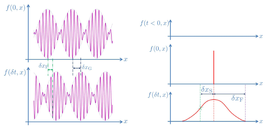
 , the phase
and group velocities are represented on the left and given respectively by
, the phase
and group velocities are represented on the left and given respectively by  and
and
 (in the limit
  .) The signal and front velocity represented on the right are
given by
.) The signal and front velocity represented on the right are
given by  (where
  is the point where at least half the intensity of the original
signal is reached.) The front velocity is given by
is the point where at least half the intensity of the original
signal is reached.) The front velocity is given by  .
.10.6.1 Superluminalities in Galileons
Superluminalities in Galileon and other closely related theories have been pointed out in several studies for more a while [412*, 1*, 262, 220, 115*, 129*, 246]. Note also that Ref. [313*] was the first work to point out the existence of superluminal propagation in the higher-dimensional picture of DGP rather than in its purely four-dimensional decoupling limit. See also Refs. [112, 110, 311, 312, 218, 219] for related discussions on super- versus sub- luminal propagation in conformal Galileon and other DBI-related models. The physical interpretation of these superluminal propagations was studied in other non-Galileon models in [199, 43*] and see [206*, 469*] for their potential connection with classicalization [214, 213, 205, 11].
In all the examples found so far, what has been pointed out is the existence of a superluminal group velocity, which is the regime inspected is the same as the phase velocity. As we will see below (see Section 10.7), in the one example where we can compute the phase velocity for momenta at which loops ought to be taken into account, we find (thanks to a dual description) that the corresponding front velocity is exactly luminal even though the low-energy group velocity is superluminal. This is no indication that all Galileon theories are causal but it comes to show how a specific Galileon theory which exhibits superluminal group velocity in some regime is dual to a causal theory.
In most of the cases considered, superluminal propagation was identified in a spherically symmetric setting in the vicinity of a localized mass as was presented in Section 10.1.2. To convince the reader that these superluminalities are independent of the coupling to matter, we show here how superluminal propagation can already occur in the vacuum in any Galileon theories without even the need of any external matter.
Consider an arbitrary quintic Galileon
where the
 are given in (6.10*) – (6.13*) and we choose the canonical normalization
  . One can
check that any plane-wave configuration of the form
is a solution of the vacuum equations of motion for any arbitrary function
. One can
check that any plane-wave configuration of the form
is a solution of the vacuum equations of motion for any arbitrary function 
 ,
with
,
with 
 , since
  for any
  for a plane-wave of the form (10.40*).
Now, considering perturbations riding on top of the plane-wave,  , these
perturbations see an effective background-dependent metric similarly as in Section 10.1.1 and have the
linearized equation of motion
, these
perturbations see an effective background-dependent metric similarly as in Section 10.1.1 and have the
linearized equation of motion

 given in (10.7*)
A perturbation traveling along the direction
given in (10.7*)
A perturbation traveling along the direction ![∑3 Zμν(π ) = (n-+-1)(n-+-2)cn+2X (n)μν(Π ) (10.43 ) 0 Λ3n 0 n[=0 ] = η μν − 12c3F ′′(x1 − t)(δμ + δμ)(δν+ δν) . (10.44 ) Λ3 0 1 0 1](article2080x.gif)
 has a velocity
  which satisfies
So, depending on wether the perturbation travels with or against the flow of the plane wave, it will have a
velocity
which satisfies
So, depending on wether the perturbation travels with or against the flow of the plane wave, it will have a
velocity 
 given by
So, a plane wave which admits26
the perturbation propagates with a superluminal velocity. However, this velocity corresponds to the group
velocity and in order to infer whether or not there is any acausality we need to derive the front
velocity, which is the large momentum limit of the phase velocity. The derivation presented here
presents a tree-level calculation and to compute the large momentum limit one would need
to include loop corrections. This is especially important as
given by
So, a plane wave which admits26
the perturbation propagates with a superluminal velocity. However, this velocity corresponds to the group
velocity and in order to infer whether or not there is any acausality we need to derive the front
velocity, which is the large momentum limit of the phase velocity. The derivation presented here
presents a tree-level calculation and to compute the large momentum limit one would need
to include loop corrections. This is especially important as 

 as the theory
becomes (infinitely) strongly coupled at that point [87*]. So far, no computation has properly
taken these quantum effects into account, and the (a)causality of Galileons theories is yet to
determined.
as the theory
becomes (infinitely) strongly coupled at that point [87*]. So far, no computation has properly
taken these quantum effects into account, and the (a)causality of Galileons theories is yet to
determined.
10.6.2 Superluminalities in massive gravity
The existence of superluminal propagation directly in massive gravity has been pointed out in many references in the literature [87*, 276*, 192*, 177*] (see also [496] for another nice discussion). Unfortunately none of these studies have qualified the type of velocity which exhibits superluminal propagation. On closer inspection it appears that there again for all the cases cited the superluminal propagation has so far always been computed classically without taking into account quantum corrections. These results are thus always valid for the low frequency group velocity but never for the front velocity which requires a fully fledged calculation beyond the tree-level classical approximation [445*].
Furthermore, while it is very likely that massive gravity admits superluminal propagation, to date there is no known consistent solution of massive gravity which has been shown to admit superluminal (even of group) velocity. We review the arguments in favor of superluminal propagation in what follows together with their limitations. Notice as well that while a Galileon theory typically admits superluminal propagation on top of static and spherically symmetric Vainshtein solutions as presented in Section 10.1.2, this is not the case for massive gravity see Section 10.1.3 and [58*].
- 1.
- Argument: Some background solutions of massive gravity admit superluminal
propagation.
Limitation of the argument: the solutions inspected were not physical.
Ref. [276] was the first work to point out the presence of superluminal group velocity in the full theory of massive gravity rather than in its Galileon decoupling limit. These superluminal modes ride on top of a solution which is unfortunately unrealistic for different reasons. First, the solution itself is unstable. Second, the solution has no rest frame (if seen as a perfect fluid) or one would need to perform a superluminal boost to bring the solution to its rest frame. Finally, to exist, such a solution should be sourced by a matter source with complex eigenvalues [142]. As a result the solution cannot be trusted in the first place, and so neither can the superluminal propagation of fluctuations about it. - 2.
- Argument: Some background solutions of the decoupling limit of massive gravity
admit superluminal propagation.
Limitation of the argument: the solutions were only found in a finite region of space and time.
In Ref. [87*] superluminal propagation was found in the decoupling limit of massive gravity. These solutions do not require any special kind of matter, however the background has only be solved locally and it has not (yet) been shown whether or not they could extrapolate to sensible and stable asymptotic solutions. - 3.
- Argument: There are some exact solutions of massive gravity for which the
determinant of the kinetic matrix vanishes thus massive gravity is acausal.
Limitation of the argument: misuse of the characteristics analysis – what has really been identified is the absence of BD ghost.
Ref. [192*] presented some solutions which appeared to admit some instantaneous modes in the full theory of massive gravity. Unfortunately the results presented in [192*] were due to a misuse of the characteristics analysis.The confusion in the characteristics analysis arises from the very constraint that eliminates the BD ghost. The existence of such a constraint was discussed in length in many different formulations in Section 7 and it is precisely what makes ghost-free (or dRGT) massive gravity special and theoretically viable. Due to the presence of this constraint, the characteristics analysis should be performed after solving for the constraints and not before [326].
In [192*] it was pointed out that the determinant of the time kinetic matrix vanished in ghost-free massive gravity before solving for the constraint. This result was then interpreted as the propagation of instantaneous modes and it was further argued that the theory was then acausal. This result is simply an artefact of not properly taking into account the constraint and performing a characteristics analysis on a set of modes which are not all dynamical (since two phase space variables are constrained by the primary and secondary constrains [295, 294]). In other word it is precisely what would–have–been the BD ghost which is responsible for canceling the determinant of the time kinetic matrix. This does not mean that the BD ghost propagates instantaneously but rather that the BD ghost is not present in that theory, which is the very point of the theory.
One can show that the determinant of the time kinetic matrix in general does not vanish when computing it after solving for the constraints. In summary the results presented in [192*] cannot be used to deduce the causality of the theory or absence thereof.
- 4.
- Argument: Massive gravity admits shock wave solutions which admit superluminal
and instantaneous modes.
Limitation of the argument: These configurations lie beyond the regime of validity of the classical theory.
Shock wave local solutions on top of which the fluctuations are superluminal were found in [177*]. Furthermore, a characteristic analysis reveals the possibility for spacelike hypersurfaces to be characteristic. While interesting, such configurations lie beyond the regime of validity of the classical theory and quantum corrections ought to be included.Having said that, it is likely that the characteristic analysis performed in [177*] and then in [178*] would give the same results had it been performed on regular solutions.27 This point is discussed below.
- 5.
- Argument: The characteristic analysis shows that some field configurations of
massive gravity admit superluminal propagation and the possibility for spacelike
hypersurfaces to be characteristic.
Limitation of the argument: Same as point 2. Putting this limitation aside this result is certainly correct classically and in complete agreement with previous results presented in the literature (see point 2 where local solutions were given).
Even though the characteristic analysis presented in [177*] used shock wave local configurations, it is also valid for smooth wave solutions which would be within the regime of validity of the theory. In [178*] the characteristic analysis for a shock wave was presented again and it was argued that CTCs were likely to exist.To better see the essence behind the general characteristic analysis argument, let us look at the (simpler yet representative) case of a Proca field with an additional quartic interaction as explored in [420*, 467],
The idea behind the characteristic analysis is to “replace the highest derivative terms by
by
 ” [420] so that one of the equations of motion is
When
” [420] so that one of the equations of motion is
When  , one can solve this equation maintaining
  . Then there are certainly field
configurations for which the normal to the characteristic surface is timelike and thus the mode with
. Then there are certainly field
configurations for which the normal to the characteristic surface is timelike and thus the mode with
 can propagate superluminally in this Proca field theory. However, as we shall see below
this very combination
can propagate superluminally in this Proca field theory. However, as we shall see below
this very combination ![𝒵 = [(m2 + λA νA ν)k αkα + 2λ(A νkν)2] = 0](article2096x.gif) with
with  timelike (say
 ) is the coefficient of the time-like kinetic term of the helicity-0 mode. So one can
never have
) is the coefficient of the time-like kinetic term of the helicity-0 mode. So one can
never have ![2 ν α ν 2 [(m + λA A ν)k kα + 2λ(A kν) ] = 0](article2099x.gif) with
with  (or any timelike
direction) without automatically having an infinitely strongly helicity-0 mode and thus
automatically going beyond the regime of validity of the theory (see Ref. [87*] for more
details.)
(or any timelike
direction) without automatically having an infinitely strongly helicity-0 mode and thus
automatically going beyond the regime of validity of the theory (see Ref. [87*] for more
details.)
To see this more precisely, let us perform the characteristic analysis in the Stückelberg language. An analysis performed in unitary gauge is of course perfectly acceptable, but to connect with previous work in Galileons and in massive gravity the Stückelberg formalism is useful.
In the Stückelberg language,
It is now clear that the combination found in the characteristic analysis , keeping track of the terms quadratic in
  , we
have
, we
have  is nothing other than
where
is nothing other than
where  is the kinetic matrix of the helicity-0 mode. Thus, a configuration with
  with
with
 implies that the
  component of helicity-0 mode kinetic matrix vanishes. This
means that the conjugate momentum associated to
component of helicity-0 mode kinetic matrix vanishes. This
means that the conjugate momentum associated to  cannot be solved for in this time-slicing, or
that the helicity-0 mode is infinitely strongly coupled.
cannot be solved for in this time-slicing, or
that the helicity-0 mode is infinitely strongly coupled.
This result should sound familiar as it echoes what has already been shown to happen in the decoupling limit of massive gravity, or here of the Proca field theory (see [43, 468] for related discussions in that case). Considering the decoupling limit of (10.48*) with
For fluctuations about a given background configuration and
and  , we obtain a decoupled massless gauge field and a scalar field,
 , the fluctuations see an
effective metric
, the fluctuations see an
effective metric  given by
Of course unsurprisingly, we find
given by
Of course unsurprisingly, we find ![&tidle;Zμν(π0) ≡ m − 2Zμν[m −1∂μπ0]](article2117x.gif) . The fact that we can find
superluminal or instantaneous propagation in the characteristic analysis is equivalent to the statement
that in the decoupling limit there exists classical field configurations for
. The fact that we can find
superluminal or instantaneous propagation in the characteristic analysis is equivalent to the statement
that in the decoupling limit there exists classical field configurations for  for which the
fluctuations propagate superluminally (or even instantaneously). Thus, the results of the characteristic
analysis are in agreement with previous results in the decoupling limit as was pointed out for instance
in [1*, 412, 87*].
for which the
fluctuations propagate superluminally (or even instantaneously). Thus, the results of the characteristic
analysis are in agreement with previous results in the decoupling limit as was pointed out for instance
in [1*, 412, 87*].
Once again, if one starts with a field configuration where the kinetic matrix is well defined, one cannot reach a region where one of the eigenvalues of
 crosses zero without going beyond the regime of
validity of the theory as described in [87*]. See also Refs. [318, 445] for the use of the characteristic
analysis and its relation to (micro-)causality.
crosses zero without going beyond the regime of
validity of the theory as described in [87*]. See also Refs. [318, 445] for the use of the characteristic
analysis and its relation to (micro-)causality.

![[ 2 ν α ν 2] μ (m + λA A ν)k kα + 2λ (A kν) k &tidle;A μ = 0. (10.49)](article2092x.gif)
![(2) 1 μν ℒ π = − -Z ∂μπ ∂νπ, (10.50) 2 with Z μν[Aμ] = ημν + -λ-A2 ημν + 2-λ-A μAν. (10.51) m2 m2](article2103x.gif)


The presence of instantaneous modes in some (self-accelerating) solutions of massive gravity was actually pointed out from the very beginning. See Refs. [139*] and [364*] for an analysis of self-accelerating solutions in the decoupling limit, and [125*] for self-accelerating solutions in the full theory (see also [264*] for a complementary analysis of self-accelerating solutions.) All these analysis had already found instantaneous modes on some self-accelerating branches of massive gravity. However, as pointed out in all these analysis, the real question is to establish whether or not these solutions lie within the regime of validity of the EFT, and whether one could reach such solutions with a finite amount of energy and while remaining within the regime of validity of the EFT.
This aspect connects with Hawking’s chronology protection argument which is already in effect in GR [302, 303], (see also [472] and [473] for a comprehensive review). This argument can be extended to Galileon theories and to massive gravity as was shown in Ref. [87*].
It was pointed out in [87*] and in many other preceding works that there exists local backgrounds in
Galileon theories and in massive gravity which admit superluminal and instantaneous propagation. (As
already mentioned, in point 2. above in massive gravity it is however unclear whether these localized
backgrounds admit stable and consistent global realizations). The worry with superluminal propagation is
that it could imply the presence of CTCs (closed timelike curves). However, when ‘cranking up’ the
background sufficiently so as to reach a solution which would admit CTCs, the Galileon or the helicity-0
mode of the graviton becomes inevitably infinitely strongly coupled. This means that the effective field
theory used breaks down and the background becomes unstable with arbitrarily fast decay time before any
CTC can ever be formed.
Summary: Several analyses have confirmed the existence of local configurations admiting superluminalities in massive gravity. At this point, we leave it to the reader’s discretion to decide whether the existence of local classical configurations which admit superluminalities and sometimes even instantaneous propagation means that the theory should be discarded. We bear in mind the following considerations:
- No stable global solutions have been found with the same properties.
- No CTCs can been constructed within the regime of validity of the theory. As shown in Ref. [87] CTCs constructed with these configurations always lie beyond the regime of validity of the theory. Indeed in order to create a CTC, a mode needs to become instantaneous. As soon as a mode becomes instantaneous, the regime of validity of the classical theory is null and classical considerations are thus obsolete.
- Finally, and most importantly, all the results presented so far for Galileons and massive gravity (including the ones summarized here), rely on classical configurations. As was explained at the beginning of this section causality is determined by the front velocity for which classical considerations break down. Therefore, no classical calculations can ever prove or disprove the (a)causality of a theory.
10.6.3 Superluminalities vs Boulware–Deser ghost vs Vainshtein
We finish by addressing what would be an interesting connection between the presence of superluminalities and the very constraint of massive gravity which removes the BD ghost which was pointed out in [192, 177, 178]. Actually, one can show that the presence of local configurations which admits superluminalities is generic to any theories of massive gravity, including DGP, cascading gravity, non-Fierz–Pauli massive gravity and even other braneworld models and is not specific to the presence of a constraint which removes the BD ghost. For instance consider a theory of massive gravity for which the cubic interactions about flat spacetime different than that of the ghost-free model of massive gravity. Then as shown in Section 2.5 (for instance, Eqs. (2.86*) or 2.89*, see also [111, 173]) the decoupling limit analysis leads to terms of the form
As we have shown earlier, results from this decoupling limit are in full agreement with a characteristic analysis.![( ) ℒFP,π = − 1-(∂π)2 + ---4--- [Π ][Π2 ] − [Π3] . (10.55 ) 2 MPlm4](article2120x.gif)
The plane wave solutions provided in (10.40*) is still a vacuum solution in this case. Following the same
analysis as that provided in Section 10.6.1, one can easily find modes propagating with superluminal group
and phase velocity for appropriate choices of functions  (while keeping within the regime of
validity of the theory.)
(while keeping within the regime of
validity of the theory.)
Alternatively, let us look a background configuration  with
with  . Without loss of
generality at any point
. Without loss of
generality at any point  one can diagonalize the matrix
  . Focusing on a mode traveling
along the
. Focusing on a mode traveling
along the  direction with momentum
  , we find the dispersion relation
![(k2 − k2) + --16---(k − k )2[k2 (¯Π0 + ¯Π2 + ¯Π3 ) + k2 (¯Π1 + ¯Π2 + ¯Π3 ) + 2k k Π¯μ ] (10.56 ) 0 1 MPlm4 0 1 1 0 2 3 0 1 2 3 0 1 μ = 0.](article2128x.gif)
 is nothing else but the signal of the BD ghost about generic
backgrounds where
is nothing else but the signal of the BD ghost about generic
backgrounds where  . Performing a characteristic analysis at this point would focus on the higher
powers in
. Performing a characteristic analysis at this point would focus on the higher
powers in  which are intrinsic to the ghost. One can follow instead the non-ghost mode which is
already present even when
which are intrinsic to the ghost. One can follow instead the non-ghost mode which is
already present even when  . To follow this mode, it is therefore sufficient to perform a
perturbative analysis in
. To follow this mode, it is therefore sufficient to perform a
perturbative analysis in  . Equation (10.56*) can always be solved for
  as well as for
We can, therefore, always find a configuration for which
as well as for
We can, therefore, always find a configuration for which 
 at least perturbatively which is sufficient
to imply the existence of superluminalities. Even if this calculation was performed perturbatively, it still
implies the presence classical superluminalities like in the previous analysis of Galileon theories or ghost-free
massive gravity.
at least perturbatively which is sufficient
to imply the existence of superluminalities. Even if this calculation was performed perturbatively, it still
implies the presence classical superluminalities like in the previous analysis of Galileon theories or ghost-free
massive gravity.
As a result the presence of local solutions in massive gravity which admit superluminalities is not connected to the constraint that removes the BD ghost. Rather it is likely that the presence of superluminalities could be tied to the Vainshtein mechanism (with flat asymptotic boundary conditions), which as we have seen is crucial for these types of theories (see Refs. [1, 313] and [129] for a possible connection.) More recently, the presence of superluminalities has also been connected to the idea of classicalization which is tied to the Vainshtein mechanism [206, 469]. It is possible that the only way these superluminalities could make sense is through this idea of classicalization. Needless to say this is very much speculative at the moment. Perhaps the Galileon dualities presented below could help understanding these open questions.
10.7 Galileon duality
The low strong coupling scale and the presence of superluminalities raises the question of how to understand the theory beyond the redressed strong coupling scale, and whether or not the superluminalities are present in the front velocity.
A non-trivial map between the conformal Galileon and the DBI conformal Galileon was recently presented in [113] (see also [55]). The conformal Galileon side admits superluminal propagation while the DBI side of the map is luminal. Since both sides are related by a ‘simple’ field redefinition which does not change the physics, and cannot change the causality of the theory, this suggests that the superluminalities encountered in that example must be in the group velocity rather than the front velocity.
Recently, another Galileon duality was proposed in [115] and [136*] by use of simple Legendre transform. First encountered within the decoupling limit of bi-gravity [224*], the duality can be seen as being related to the freedom in how to introduce the Stückelberg fields. However, the duality survives independently from bi-gravity and could be significant in the context of massive gravity.
To illustrate this duality, we start with a full Galileon in  dimensions as in (10.6*)
![( ) ∫ ∑d cn+1 S = ddx π -3(n−1)ℒn[Π ] , (10.58 ) n=1 Λ](article2138x.gif)
In terms of the dual field  , the Galileon theory (10.58*) is nothing other than another Galileon
with different coefficients,
, the Galileon theory (10.58*) is nothing other than another Galileon
with different coefficients,
![∫ ( d ) d ∑ -pn+1-- S = d &tidle;x ρ(&tidle;x) Λ3(n−1)ℒn [Σ ] , (10.63 ) n=1](article2142x.gif)
 and the new coefficients are given by [136]
This duality thus maps a Galileon to another Galileon theory with different coefficients. In particular this
means that the free theory
and the new coefficients are given by [136]
This duality thus maps a Galileon to another Galileon theory with different coefficients. In particular this
means that the free theory 
 maps to another non-trivial
  order Galileon theory with
 for any
  . This dual Galileon theory admits superluminal propagation precisely in
the same way as was pointed out on the spherically symmetric configurations of Section 10.1.2 or on the
plane wave solutions of Section 10.6.1. Yet, this non-trivial Galileon is dual to a free theory which is causal
and luminal by definition.
. This dual Galileon theory admits superluminal propagation precisely in
the same way as was pointed out on the spherically symmetric configurations of Section 10.1.2 or on the
plane wave solutions of Section 10.6.1. Yet, this non-trivial Galileon is dual to a free theory which is causal
and luminal by definition.
What was computed in these examples for a non-trivial Galileon theory (and in all the examples known so far in the literature) is only the tree-level group velocity valid till the (redressed) strong coupling scale of the theory. Once hitting the (redressed) strong coupling scale the loops need to be included. In the dual free theory however there are no loops to account for, and thus the result of luminal velocity in that free theory is valid at all scale and has to match the front velocity. This is strongly suggestive that the front velocity in that example of non-trivial Galileon theory is luminal and the theory is causal even though it exhibits a superluminal group velocity.
It is clear at this point that a deeper understanding of this class of theories is required. We expect this will be the subject of further studies. In the rest of this review, we focus on some phenomenological aspects of massive gravity before presenting other theories of massive gravity.
 |
 |
 |
Living Rev. Relativity, 17 (2014), 7, doi:10.12942/lrr-2014-7, URL (accessed <date>): http://www.livingreviews.org/lrr-2014-7.
 This work is licensed under a Creative Commons License.
© The author(s), except where otherwise noted.
This work is licensed under a Creative Commons License.
© The author(s), except where otherwise noted.