 -decoupling
limit of bi-gravity
-decoupling
limit of bi-gravity
 )
)11 Phenomenology
Below, we summarize some of the phenomenology of massive gravity and DGP. Many other interesting results have been derived in the literature, including the implication for the very Early Universe. For instance false vacuum decay and the Hartle–Hawking no-boundary proposal was studied in the context of massive gravity in [498, 439, 499] where it was shown that the graviton mass could increase the rate. The implications of massive gravity to the cyclic Universe were also studied in Ref. [91] with a regular bounce. We emphasize that in massive gravity the reference metric has to be chosen once and for all and cannot be modified, no matter what the background configuration is (no matter whether we are interested in cosmology, or in spherically symmetry configurations or other). This is a consistent procedure since massive gravity has been shown to be free of the BD ghost for any choice of reference metric independently of the background configuration. Theories with different reference metrics represent different independent theories.
11.1 Gravitational waves
11.1.1 Speed of propagation
If the photon had a mass it would no longer propagate at ‘the speed of light’, but at a lower speed. For the
photon its speed of propagation is known with such an accuracy in so many different media that it can be
used to put the most stringent constraints on the photon mass to [68]  . In the rest of this
review we will adopt the viewpoint that the photon is massless and that light does indeed propagate at the
‘speed of light’.
. In the rest of this
review we will adopt the viewpoint that the photon is massless and that light does indeed propagate at the
‘speed of light’.
The earliest bounds on the graviton mass were based on the same idea. As described in [487*], (see
also [394]), if the graviton had a mass, gravitational waves would propagate at a speed different than that
of light,  (assuming a speed of light
  ). This different velocity between the
light and gravitational waves would manifest itself in observations of supernovae. Assuming the
emission of a gravitational wave with frequency larger than the graviton mass, this could lead to
a bound on the graviton mass of
). This different velocity between the
light and gravitational waves would manifest itself in observations of supernovae. Assuming the
emission of a gravitational wave with frequency larger than the graviton mass, this could lead to
a bound on the graviton mass of  considering a frequency of 100 Hz and a
supernovae located 200 Mpc away [487*] (assuming that the photon propagates at the speed of
light).
considering a frequency of 100 Hz and a
supernovae located 200 Mpc away [487*] (assuming that the photon propagates at the speed of
light).
Alternatively, another way to test the speed of gravitational waves and bound the graviton mass
without relying on any assumptions on the photon is through the observation of inspiralling
compact objects which allows to derive the frequency-dependence of GWs. The detection of
GWs in Advanced LIGO could then bound the graviton mass potentially all the way down to
 [487*, 486, 71].
The graviton mass is also relevant for the production of primordial gravitational waves during inflation. Following the analysis of [282] it was shown that the graviton mass opens up the production of gravitational waves during inflation with a sharp peak with a height and position which depend on the graviton mass. See also [403] for the study of exact plane wave solutions in massive gravity.
Nevertheless, these bounds on the graviton mass are relatively weak compared to the typical value of
 considered till now in this review. The reason for this is because these bounds do
not take into account the effects arising from the additional polarization in the gravitational waves which
would be present if the graviton had a mass in a Lorentz-invariant theory. For the photon, if it had a
mass, the additional polarization would decouple and would therefore be irrelevant (this is
related to the absence of vDVZ discontinuity at the classical level for a Proca theory.) In massive
gravity, however, the helicity-0 mode of the graviton couples to matter. As we shall see below, the
bounds on the graviton mass inferred from the absence of fifth forces are typically much more
stringent.
considered till now in this review. The reason for this is because these bounds do
not take into account the effects arising from the additional polarization in the gravitational waves which
would be present if the graviton had a mass in a Lorentz-invariant theory. For the photon, if it had a
mass, the additional polarization would decouple and would therefore be irrelevant (this is
related to the absence of vDVZ discontinuity at the classical level for a Proca theory.) In massive
gravity, however, the helicity-0 mode of the graviton couples to matter. As we shall see below, the
bounds on the graviton mass inferred from the absence of fifth forces are typically much more
stringent.
11.1.2 Additional polarizations
One of the predictions of GR is the existence of gravitational waves (GW) with two transverse independent polarizations.
While GWs have not been directly detected via interferometer yet, they have been detected through the spin-down of binary pulsar systems [322, 457, 485]. This detection via binary pulsars does not count as a direct detection, but it matches expectations from GWs with such an accuracy, and for now so many different systems of different relative masses that it seems unlikely that the spin-down could be due to something different than the emission of GWs.
In a modified theory of gravity, one could expect a total of up to six polarizations for the GWs as seen in Figure 6*.
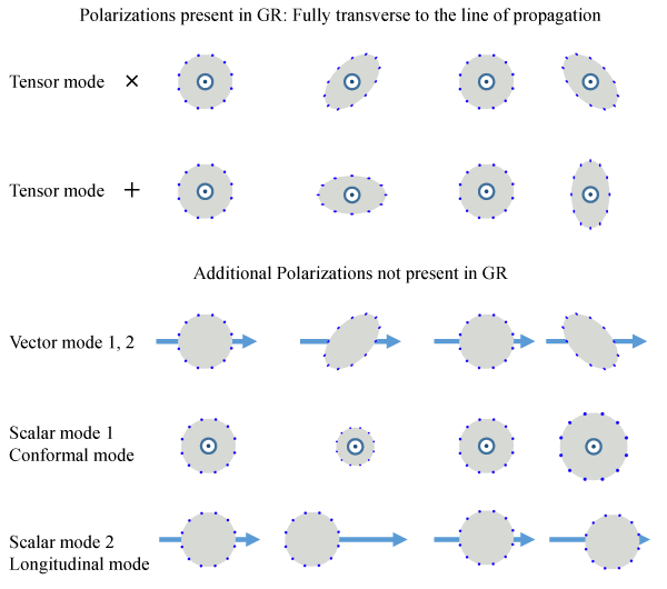
As emphasized in the first part of this review, and particularly in Section 2.5, the sixth excitation, namely the longitudinal one, represents a ghost degree of freedom. Thus, if that mode is observed, it cannot be arising from a Lorentz-invariant massive graviton. Its presence could be linked for instance to new scalar degrees of freedom which are independent from the graviton itself. In massive gravity, only five polarizations are expected. Notice however that the helicity-1 mode does not couple directly to matter or external sources, so it is unlikely that GWs with polarizations which mix the transverse and longitudinal directions would be produced in a natural process.
Furthermore, any physical process which is expected to produce GWs would include very dense sources where the Vainshtein mechanism will thus be expected to be active and screen the effect of the helicity-0 mode. As a result the excitation of the breathing mode is expected to be suppressed in any theory of massive gravity which includes an active Vainshtein mechanism.
So, while one could in principle expect up to six polarizations for GWs in a modified theory of gravity, in massive gravity only the two helicity-2 polarizations are expected to be produced in a potentially observable amount by interferometers like advanced-LIGO [289]. To summarize, in ghost-free massive gravity or DGP we expect the following:
- The helicity-2 modes are produced in the same way as in GR and would be indistinguishable if they travel distances smaller than the graviton Compton wavelength
- The helicity-1 modes are not produced
- The breathing or conformal mode is produced but suppressed by the Vainshtein mechanism and so the magnitude of this mode is suppressed compared to the helicity-2 polarization by many orders of magnitudes.
- The longitudinal mode does not exist in a ghost-free theory of massive gravity. If such a mode is observed it must be arise from another field independent from the graviton.
We will also discuss the implications for indirect detection of GWs via binary pulsar spin-down in Section 11.4. We will see that already in these setups the radiation in the breathing mode is suppressed by 8 orders of magnitude compared to that in the helicity-2 mode. In more relativistic systems such as black-hole mergers, this suppression will be even bigger as the Vainshtein mechanism is stronger in these cases, and so we do not expect to see the helicity-0 mode component of a GW emitted by such systems.
To summarize, while additional polarizations are present in massive gravity, we do not expect to be able to observe them in current interferometers. However, these additional polarizations, and in particular the breathing mode can have larger effects on solar-system tests of gravity (see Section 11.2) as well as for weak lensing (see Section 11.3), as we review in what follows. They also have important implications for black holes as we discuss in Section 11.5 and in cosmology in Section 12.
11.2 Solar system
A lot of the phenomenology of massive gravity can be derived from its decoupling limit where it resembles a Galileon theory. Since the Galileon was first encountered in DGP most of the phenomenology was first derived for that model. The extension to massive gravity is usually relatively straightforward with a few subtleties which we mention at the end. We start by reviewing the phenomenology assuming a cubic Galileon decoupling limit, which is directly applicable for DGP and then extend to the quartic Galileon and ghost-free massive gravity.
Within the context of DGP, a lot of its phenomenology within the solar system was derived in [388*, 386*] using the full higher-dimensional picture as well as in [215*]. In these work the effect from the helicity-0 mode in the advanced of the perihelion were computed explicitly. In particular in [215*] it was shown how an infrared modification of gravity could have an effect on small solar system scales and in particular on the Moon. In what follows we review their approach.
Consider a point source of mass  localized at
  . In GR (or rather Newtonian gravity as
it is a sufficient approximation), the gravitational potential mediated by the point source is
. In GR (or rather Newtonian gravity as
it is a sufficient approximation), the gravitational potential mediated by the point source is

 is the Schwarzschild radius associated with the source. Now, in a theory of massive gravity, the
helicity-0 mode of the graviton also contributes to the gravitational potential with an additional amount
is the Schwarzschild radius associated with the source. Now, in a theory of massive gravity, the
helicity-0 mode of the graviton also contributes to the gravitational potential with an additional amount
 . As seen in Section 10.1, when the Vainshtein mechanism is active the contribution from the
helicity-0 mode is very much suppressed.
. As seen in Section 10.1, when the Vainshtein mechanism is active the contribution from the
helicity-0 mode is very much suppressed.  but measurements in the Solar system
are reaching such a level of accuracy than even a small deviation
but measurements in the Solar system
are reaching such a level of accuracy than even a small deviation  could in principle be
observable [488*].
could in principle be
observable [488*].
In the decoupling limit of DGP, matter fields couple to the following perturbed metric
where
 is the helicity-0 mode of the graviton (up to some dimensionless numerical factors which we have
set to unity). In massive gravity, matter couples to the following metric (see the discussion in Section 10.1.3
and (10.21*)),
The deviation
is the helicity-0 mode of the graviton (up to some dimensionless numerical factors which we have
set to unity). In massive gravity, matter couples to the following metric (see the discussion in Section 10.1.3
and (10.21*)),
The deviation 
 to the gravitational potential is thus given by
(notice that in the static and spherically symmetric case
to the gravitational potential is thus given by
(notice that in the static and spherically symmetric case 
 leads to no correction to the
gravitational potential).
leads to no correction to the
gravitational potential).
Following [215*] we define as  the fractional change in the gravitational potential

 (of for instance the Earth) as compared to GR. For
elliptical orbits this leads to an additional angular precession of the perihelion due to the force mediated by
the helicity-0 mode on top of that of GR. The additional advanced of the perihelion per orbit is given in
terms of
(of for instance the Earth) as compared to GR. For
elliptical orbits this leads to an additional angular precession of the perihelion due to the force mediated by
the helicity-0 mode on top of that of GR. The additional advanced of the perihelion per orbit is given in
terms of  as
where
as
where 
 is the mean orbit radius, (notice the
  in that expression is the standard value
  nothing to do with the helicity-0 mode).
DGP and cubic Galileon
In the decoupling limit of DGP (cubic Galileon)  was given in (10.15*) and
  , where
 is the strong coupling radius derived in (10.14*),
  leading to an anomalous
advance of the perihelion
leading to an anomalous
advance of the perihelion
 and the departure from GR goes to zero, this is another
example of how the Vainshtein mechanism arises. Interestingly, it was pointed out in [388*, 386*] that in
DGP the sign of this anomalous angle depends on whether on the branch studied (self-accelerating branch –
or normal branch).
and the departure from GR goes to zero, this is another
example of how the Vainshtein mechanism arises. Interestingly, it was pointed out in [388*, 386*] that in
DGP the sign of this anomalous angle depends on whether on the branch studied (self-accelerating branch –
or normal branch).
For the Earth-Moon system, taking  with
with  , this leads to an
anomalous precision of the order of [215*]
, this leads to an
anomalous precision of the order of [215*]

 /year
/year  /orbit).
As pointed out in [215] and [388, 386], the effect could be bigger for the advance of the perihelion of Mars around the Sun, but at the moment the accuracy is slightly less.
Massive gravity and quartic Galileon:
As already mentioned in Section 10.1.2, the Vainshtein mechanism is typically much stronger28 in the spherically symmetric configuration of the quartic Galileon and thus in massive gravity (see for instance the suppression of the force given in (10.17*)). Using the same values as before for a quartic Galileon we obtain
Furthermore, in massive gravity the parameter that enters this relation is not directly the graviton but rather the graviton mass weighted with the coefficient
 which depends on the
cubic potential term
which depends on the
cubic potential term  , assuming that
  , (see Section 10.1.3 for more precision)
This is typically very far from observations unless we are very close to the minimal
model.29
, (see Section 10.1.3 for more precision)
This is typically very far from observations unless we are very close to the minimal
model.29

11.3 Lensing
As mentioned previously, one peculiarity of massive gravity not found in DGP nor in a typical Galileon
theory (unless we derive the Galileons from a higher-dimensional brane picture [157]) is the new disformal
coupling to matter of the form  , which means that the helicity-0 mode also couples to
conformal matter.
, which means that the helicity-0 mode also couples to
conformal matter.
In the vacuum, for a static and spherically symmetric configuration the coupling  plays no
role. So to the level at which we are working when deriving the Vainshtein mechanism about a point-like
mass this additional coupling to matter does not affect the background configuration of the field (see [140]
for a discussion outside the vacuum, taking into account for the instance the effect of the Earth
atmosphere). However, it does affect this disformal coupling does affect the effect metric seen by
perturbed sources on top of this configuration. This could have some implications for structure
formation is to the best of our knowledge have not been fully explored yet, and does affect the
bending of light. This effect was pointed out in [490*] and the effects to gravitational lensing were
explored. We review the key results in what follows and refer to [490*] for further discussions (see
also [448]).
plays no
role. So to the level at which we are working when deriving the Vainshtein mechanism about a point-like
mass this additional coupling to matter does not affect the background configuration of the field (see [140]
for a discussion outside the vacuum, taking into account for the instance the effect of the Earth
atmosphere). However, it does affect this disformal coupling does affect the effect metric seen by
perturbed sources on top of this configuration. This could have some implications for structure
formation is to the best of our knowledge have not been fully explored yet, and does affect the
bending of light. This effect was pointed out in [490*] and the effects to gravitational lensing were
explored. We review the key results in what follows and refer to [490*] for further discussions (see
also [448]).
In GR, the relevant potential for lensing is  , where we use the same
notation as before,
, where we use the same
notation as before,  and
and  . A conformal coupling of the form
  does not affect
this lensing potential but the disformal coupling
does not affect
this lensing potential but the disformal coupling  leads to a new contribution
  given by

 .] This new contribution to the lensing
potential leads to an anomalous fractional lensing of
For the bending of light about the Sun, this leads to an effect of the order of
which is utterly negligible. Note that this is a tree-level calculation. When getting at these distances loops
ought to be taken into account as well.
.] This new contribution to the lensing
potential leads to an anomalous fractional lensing of
For the bending of light about the Sun, this leads to an effect of the order of
which is utterly negligible. Note that this is a tree-level calculation. When getting at these distances loops
ought to be taken into account as well.


At the level of galaxies or clusters of galaxy, the effect might be more tangible. The reason for that is that for the mass of a galaxy, the associated strong coupling radius is not much larger than the galaxy itself and thus at the edge of a galaxy these effects could be stronger. These effects were investigated in [490] where it was shown a few percent effect on the tangential shear caused by the helicity-0 mode of the graviton or of a disformal Galileon considering a Navarro–Frenk–White halo profile, for some parameters of the theory. Interestingly, the effect peaks at some specific radius which is the same for any halo when measured in units of the viral radius. Even though the effect is small, this peak could provide a smoking gun for such modifications of gravity.
Recently, another analysis was performed in Ref. [407], where the possibility to testing theories of modified gravity exhibiting the Vainshtein mechanism against observations of cluster lensing was explored. In such theories, like in massive gravity, the second derivative of the field can be large at the transition between the screened and unscreened region, leading to observational signatures in cluster lensing.
11.4 Pulsars
One of the main predictions of massive gravity is the presence of new polarizations for GWs. While these new polarization might not be detectable in GW interferometers as explained in Section 11.1.2, we could still expect them to lead to detectable effects in the binary pulsar systems whose spin-down is in extremely good agreement with GR. In this section, we thus consider the power emitted in the helicity-0 mode of the graviton in a binary-pulsar system. We use the effective action approach derived by Goldberger and Rothstein in [254] and start with the decoupling limit of DGP before exploring that of ghost-free massive gravity and discussing the subtleties that arise in that case. We mainly focus on the monopole and quadrupole radiation although the whole formalism can be derived for any multipoles. We follow the derivation of Refs. [158*, 151*], see also Refs. [100, 18] for related studies.
In order to account for the Vainshtein mechanism into account we perform a similar
background-perturbation split as was performed in Section 10.1. The source is thus split as
 where
where  is a static and spherically source representing the total mass localized at the
center of mass and
is a static and spherically source representing the total mass localized at the
center of mass and  captures the motion of the companions with respect to the center of
mass.
captures the motion of the companions with respect to the center of
mass.
This matter profile leads to a profile for the helicity-0 mode (here mimicked as a cubic Galileon which is
the case for DGP) as in (10.3*) as  , where the background
  has the same static and
spherical symmetry as
has the same static and
spherical symmetry as  and so has the same profile as in Section 10.1.2.
The background configuration  of the field was derived in (10.13*) where
  accounts in
this case for the total mass of both companions and
accounts in
this case for the total mass of both companions and  is the distance to the center of mass.
Following the same procedure, the fluctuation
is the distance to the center of mass.
Following the same procedure, the fluctuation  then follows a modified Klein–Gordon equation

 and
and  in the vicinity of the binary pulsar system (well within the strong coupling radius defined
in (10.14*).)
in the vicinity of the binary pulsar system (well within the strong coupling radius defined
in (10.14*).)
Expanding the field in spherical harmonics the mode functions satisfy
where the modes are normalized so as to satisfy the standard normalization in the WKB region, for![2[ −iωt] Z (π0)∂x u ℓ(r)Y ℓm (Ω)e = 0, (11.15 )](article2220x.gif)
 .
.
The total power emitted via the field  is given by the sum over these mode functions,

 is the orbital period of the binary system and
  is the corresponding angular
velocity.
is the corresponding angular
velocity.  is the power emitted in the monopole,
  in the dipole
  in the quadrupole of the
field
in the quadrupole of the
field  uniquely, etc…in addition to the standard power emitted in the helicity-2 quadrupole channel of
GR.
uniquely, etc…in addition to the standard power emitted in the helicity-2 quadrupole channel of
GR.
Without the Vainshtein mechanism, the mode functions would be the same as for a standard
free-field in flat space-time,  and the power emitted in the monopole would
be larger than that emitted in GR, which would be clearly ruled out by observations. The
Vainshtein mechanism is thus crucial here as well for the viability of DGP or ghost-free massive
gravity.
and the power emitted in the monopole would
be larger than that emitted in GR, which would be clearly ruled out by observations. The
Vainshtein mechanism is thus crucial here as well for the viability of DGP or ghost-free massive
gravity.
Monopole
Taking the prefactor  into account, the zero mode for the monopole is given instead by

 which is the region where the radiation would be emitted. As
a result, the power emitted in the monopole channel through the field
which is the region where the radiation would be emitted. As
a result, the power emitted in the monopole channel through the field  is given by [158]
where
is given by [158]
where 
 is the reduced mass and
  is the semi-major axis of the orbit and
  is a numerical prefactor
of order 1 which depends on the eccentricity of the orbit.
is a numerical prefactor
of order 1 which depends on the eccentricity of the orbit.
This is to be compared with the Peters–Mathews formula for the power emitted in GR (in the helicity-2 modes) in the quadrupole [428],
where
 is again a different numerical prefactor which depends on the eccentricity of the orbit, and
  is a different combination of the companion masses, when both masses are the same (as is almost the case
for the Hulse–Taylor pulsar),
is a different combination of the companion masses, when both masses are the same (as is almost the case
for the Hulse–Taylor pulsar),  .
.
We see that the radiation in the monopole is suppressed by a factor of  compared with the
GR result. For the Hulse–Taylor pulsar this is a suppression of 10 orders of magnitudes which is completely
unobservable (at best the precision of the GR result is of 3 orders of magnitude).
compared with the
GR result. For the Hulse–Taylor pulsar this is a suppression of 10 orders of magnitudes which is completely
unobservable (at best the precision of the GR result is of 3 orders of magnitude).
Notice, however, that the suppression is far less than what was naively anticipated from the static approximation in Section 10.1.2.
The same analysis can be performed for the dipole emission with an even larger suppression of about 19 orders of magnitude compared the Peters–Mathews formula.
Quadrupole
The quadrupole emission in the field  is slightly larger than the monopole. The reason is that energy
conservation makes the non-relativistic limit of the monopole radiation irrelevant and one needs to take the
first relativistic correction into account to emit in that channel. This is not so for the quadrupole as it does
not correspond to the charge associated with any Noether current even in the non-relativistic
limit.
is slightly larger than the monopole. The reason is that energy
conservation makes the non-relativistic limit of the monopole radiation irrelevant and one needs to take the
first relativistic correction into account to emit in that channel. This is not so for the quadrupole as it does
not correspond to the charge associated with any Noether current even in the non-relativistic
limit.
In the non-relativistic limit, the mode function for the quadrupole is simply
 yielding a quadrupole emission

 is another numerical factor which depends on the eccentricity of the orbit and
  another
reduced mass. The Vainshtein suppression in the quadrupole is
another
reduced mass. The Vainshtein suppression in the quadrupole is  for the
Hulse–Taylor pulsar, and is thus well below the limit of being detectable.
for the
Hulse–Taylor pulsar, and is thus well below the limit of being detectable.
Quartic Galileon
When extending the analysis to more general Galileons or to massive gravity which includes a quartic
Galileon, we expect a priori by following the analysis of Section 10.1.2, to find a stronger Vainshtein
suppression. This result is indeed correct when considering the power radiated in only one multipole. For
instance in a quartic Galileon, the power emitted in the field  via the quadrupole channel is suppressed
by 12 orders of magnitude compared the GR emission.
via the quadrupole channel is suppressed
by 12 orders of magnitude compared the GR emission.
However, this estimation does not account for the fact that there could be many multipoles contributing with the same strength in a quartic Galileon theory [151].
In a quartic Galileon theory, the effective metric in the strong coupling radius for a static and spherically symmetric background is
the fact that the angular direction is not suppressed by
 but rather by a constant
  implies that the
multipoles are no longer suppressed by additional powers of velocity as is the case in GR or in the cubic
Galileon. This implies that many multipoles contribute with the same strength, yielding a potentially large
results. This is a sign that perturbation theory is not under control on top of this static and spherically
symmetric background and one should really consider a more realistic background which will resume some
of these contributions.
implies that the
multipoles are no longer suppressed by additional powers of velocity as is the case in GR or in the cubic
Galileon. This implies that many multipoles contribute with the same strength, yielding a potentially large
results. This is a sign that perturbation theory is not under control on top of this static and spherically
symmetric background and one should really consider a more realistic background which will resume some
of these contributions.
In situations where there is a large hierarchy between the mass of the two objects (which is the case for instance within the solar system), perturbation theory can be seen to remain under control and the power emitted in the quartic Galileon is completely negligible.
11.5 Black holes
As in any gravitational theory, the existence and properties of black holes are crucially important for probing the non-perturbative aspects of gravity. The celebrated black-hole theorems of GR play a significant role in guiding understanding of non-perturbative aspects of quantum gravity. Furthermore, the phenomenology of black holes is becoming increasingly important as understanding of astrophysical black holes increases.
Massive gravity and its extensions certainly exhibit black-hole solutions and if the Vainshtein mechanism is successful then we would expect solutions which look arbitrary close to the Schwarzschild and Kerr solutions of GR. However, as in the case of cosmological solutions, the situation is more complicated due to the absence of a unique static spherically symmetric solution that arises from the existence of additional degrees of freedom, and also the existence of other branches of solutions which may or may not be physical. There are a handful of known exact solutions in massive gravity [413*, 363*, 365*, 277*, 105*, 56*, 477*, 90, 478*, 455*, 30*, 357*], but the most interesting and physically relevant solutions probably correspond to the generic case where exact analytic solutions cannot be obtained. A recent review of black-hole solutions in bi-gravity and massive gravity is given in [478*].
An interesting effect was recently found in the context of bi-gravity in Ref. [41]. In that case, the Schwarzschild solutions were shown to be unstable (with a Gregory–Laflamme type of instability [268, 269]) at a scale dictated by the graviton mass, i.e., the instability rate is of the order of the age of the Universe. See also Ref. [42] where the analysis was generalized to the non-bidiagonal. In this more general situation, spherically symmetric perturbations were also found but generically no instabilities. Black-hole disappearance in massive gravity was explored in Ref. [401].
Since all black-hole solutions of massive gravity arise as decoupling limits  of solutions in
bi-gravity,30
we can consider from the outset the bi-gravity solutions and consider the massive gravity limit after the
fact. Let us consider then the bi-gravity action expressed as
of solutions in
bi-gravity,30
we can consider from the outset the bi-gravity solutions and consider the massive gravity limit after the
fact. Let us consider then the bi-gravity action expressed as
![∫ ∫ M-2Pl 4 √ --- M-2f- 4 ∘ ---- S = 2 d x − gR [g] + 2 d x − f R[f] (11.22 ) 2 2 ∫ ∑ √ -- + m--M-eff d4x √ − g βnℒ ( 𝕏 ) + Matter, 4 n! n n](article2256x.gif)
 . Here, the definition is such that in the limit
  the
the  ’s
correspond the usual expressions in massive gravity. We may imagine matter coupled to both metrics
although to take the massive gravity limit we should imagine black holes formed from matter which
exclusively couples to the
’s
correspond the usual expressions in massive gravity. We may imagine matter coupled to both metrics
although to take the massive gravity limit we should imagine black holes formed from matter which
exclusively couples to the  metric.
One immediate consequence of working with bi-gravity is that since the  metric is sourced by
polynomials of
metric is sourced by
polynomials of  whereas the
  metric is sourced by polynomials of
  . We, thus,
require that
. We, thus,
require that  is invertible away from curvature singularities. This is equivalent to saying that the
eigenvalues of
is invertible away from curvature singularities. This is equivalent to saying that the
eigenvalues of  and
and  should not pass through zero away from a curvature singularity. This in
turn means that if one metric is diagonal and admits a horizon, the second metric if it is diagonal must
admit a horizon at the same place, i.e., two diagonal metrics have common horizons. This is a generic
observation that is valid for any theory with more than one metric [167*] regardless of the field
equations. Equivalently, this implies that if
should not pass through zero away from a curvature singularity. This in
turn means that if one metric is diagonal and admits a horizon, the second metric if it is diagonal must
admit a horizon at the same place, i.e., two diagonal metrics have common horizons. This is a generic
observation that is valid for any theory with more than one metric [167*] regardless of the field
equations. Equivalently, this implies that if  is a diagonal metric without horizons, e.g.,
Minkowski spacetime, then the metric for a black hole must be non-diagonal when working
in unitary gauge. This is consistent with the known exact solutions. For certain solutions it
may be possible by means of introducing Stückelberg fields to put both metrics in diagonal
form, due to the Stückelberg fields absorbing the off-diagonal terms. However, for the generic
solution we would expect that at least one metric to be non-diagonal even with Stückelberg fields
present.
is a diagonal metric without horizons, e.g.,
Minkowski spacetime, then the metric for a black hole must be non-diagonal when working
in unitary gauge. This is consistent with the known exact solutions. For certain solutions it
may be possible by means of introducing Stückelberg fields to put both metrics in diagonal
form, due to the Stückelberg fields absorbing the off-diagonal terms. However, for the generic
solution we would expect that at least one metric to be non-diagonal even with Stückelberg fields
present.
Working with a static spherically symmetric ansatz for both metrics, we find in general that bi-gravity admits Schwarzschild-(anti) de Sitter-type metrics of the form (see [478*] for a review)
where are the familiar metric functions for de Sitter and Schwarzschild–de Sitter.
The  -metric coordinates are related to those of the
  metric by (in other words the profiles of the
Stückelberg fields)
metric by (in other words the profiles of the
Stückelberg fields)

 is given by
Finally, the two effective cosmological constants that arise from the mass terms are
In this form, we see that in the limit
is given by
Finally, the two effective cosmological constants that arise from the mass terms are
In this form, we see that in the limit 
 we have
  and
and  and then these
solutions match onto the known exact black holes solutions in massive gravity in the absence
of charge [413, 363*, 365, 277, 105, 56, 477*, 478*, 455*, 30, 357]. Note in particular that for
every set of
and then these
solutions match onto the known exact black holes solutions in massive gravity in the absence
of charge [413, 363*, 365, 277, 105, 56, 477*, 478*, 455*, 30, 357]. Note in particular that for
every set of  ’s there are two branches of solutions determined by the two possible values of
 .
.
These solutions describe black holes sourced by matter minimally coupled to metric  with mass
  .
An obvious generalization is to assume that the matter couples to both metrics, with effective masses
.
An obvious generalization is to assume that the matter couples to both metrics, with effective masses  and
and  so that
 are five functions of radius that are numerically obtained solutions of
five differential equations. According to the previous arguments about diagonal metrics [167*]
these solutions do not correspond to black holes in the massive gravity on Minkowski limit
are five functions of radius that are numerically obtained solutions of
five differential equations. According to the previous arguments about diagonal metrics [167*]
these solutions do not correspond to black holes in the massive gravity on Minkowski limit
 , however the limit
  can be taken and they correspond to black-hole solutions
in a theory of massive gravity in which the reference metric is Schwarzschild (–de Sitter or
anti-de Sitter). The arguments of [167] are then evaded since the reference metric itself admits a
horizon.
can be taken and they correspond to black-hole solutions
in a theory of massive gravity in which the reference metric is Schwarzschild (–de Sitter or
anti-de Sitter). The arguments of [167] are then evaded since the reference metric itself admits a
horizon.
 |
 |
 |
Living Rev. Relativity, 17 (2014), 7, doi:10.12942/lrr-2014-7, URL (accessed <date>): http://www.livingreviews.org/lrr-2014-7.
 This work is licensed under a Creative Commons License.
© The author(s), except where otherwise noted.
This work is licensed under a Creative Commons License.
© The author(s), except where otherwise noted.