 -decoupling
limit of bi-gravity
-decoupling
limit of bi-gravity
 )
)List of Figures
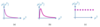 |
Figure 1:
Spectral representation of different models. (a) DGP (b) higher-dimensional cascading gravity and (c) multi-gravity. Bi-gravity is the special case of multi-gravity with one massless mode and one massive mode. Massive gravity is the special case where only one massive mode couples to the rest of the standard model and the other modes decouple. (a) and (b) are models of soft massive gravity where the graviton mass can be thought of as a resonance. |
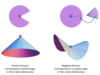 |
Figure 2:
Codimension-2 brane with positive (resp. negative) tension brane leading to a positive (resp. negative) deficit angle in the two extra dimensions. |
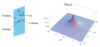 |
Figure 3:
Seven-dimensional cascading scenario and solution for one the metric potential  on
the on
the  -dimensional brane in a 7-dimensional cascading gravity scenario with tension on the -dimensional brane in a 7-dimensional cascading gravity scenario with tension on the
 -dimensional brane located at -dimensional brane located at  , in the case where , in the case where  . .
 and and  represent the two extra dimensions on the represent the two extra dimensions on the  -dimensional brane. Image
reproduced with permission from [149], copyright APS. -dimensional brane. Image
reproduced with permission from [149], copyright APS. |
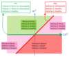 |
Figure 4:
Degrees of freedom for massive gravity on a maximally symmetric reference metric. The only theoretically allowed regions are the upper left green region and the line  corresponding
to GR. corresponding
to GR. |
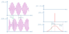 |
Figure 5:
Difference between phase, group, signal and front velocities. At  , the phase
and group velocities are represented on the left and given respectively by , the phase
and group velocities are represented on the left and given respectively by  and and
 (in the limit (in the limit  .) The signal and front velocity represented on the right are
given by .) The signal and front velocity represented on the right are
given by  (where (where  is the point where at least half the intensity of the original
signal is reached.) The front velocity is given by is the point where at least half the intensity of the original
signal is reached.) The front velocity is given by  . . |
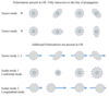 |
Figure 6:
Polarizations of gravitational waves in general relativity and potential additional polarizations in modified gravity. |
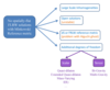 |
Figure 7:
Alternative ways in deriving the cosmology in massive gravity. |
Claudia de Rham, "Massive Gravity",
Living Rev. Relativity, 17 (2014), 7, doi:10.12942/lrr-2014-7, URL (accessed <date>): http://www.livingreviews.org/lrr-2014-7. This work is licensed under a Creative Commons License.
© The author(s), except where otherwise noted.
This work is licensed under a Creative Commons License.
© The author(s), except where otherwise noted.
Living Rev. Relativity, 17 (2014), 7, doi:10.12942/lrr-2014-7, URL (accessed <date>): http://www.livingreviews.org/lrr-2014-7.
This work is licensed under a Creative Commons License.
© The author(s), except where otherwise noted.