 -decoupling
limit of bi-gravity
-decoupling
limit of bi-gravity
 )
)8 Decoupling Limits
8.1 Scaling versus decoupling
Before moving to the decoupling of massive gravity and bi-gravity, let us make a brief interlude concerning the correct identification of degrees of freedom. The Stückelberg trick used previously to identify the correct degrees of freedom works in all generality, but care must be used when taking a “decoupling limit” (i.e., scaling limit) as will be done in Section 8.2.
Imagine the following gauge field theory
i.e., the Proca mass term without any kinetic Maxwell term for the gauge field. Since there are no dynamics in this theory, there is no degrees of freedom. Nevertheless, one could still proceed and use the same split
 as performed previously,
so as to introduce what appears to be a kinetic term for the mode
as performed previously,
so as to introduce what appears to be a kinetic term for the mode 
 . At this level the theory is still
invariant under
. At this level the theory is still
invariant under  and
and  , and so while there appears to be a dynamical degree
of freedom
, and so while there appears to be a dynamical degree
of freedom  , the symmetry makes that degree of freedom unphysical, so that (8.2*) still propagates no
physical degree of freedom.
, the symmetry makes that degree of freedom unphysical, so that (8.2*) still propagates no
physical degree of freedom.
Now consider the  scaling limit of (8.2*) while keeping
  and
and  finite. In that scaling
limit, the theory reduces to
finite. In that scaling
limit, the theory reduces to

 fixed but rather with
  fixed.
This is indeed a consistent rescaling which leads to finite contributions in the limit
fixed.
This is indeed a consistent rescaling which leads to finite contributions in the limit  ,
which clearly propagates no degrees of freedom.
,
which clearly propagates no degrees of freedom.

This procedure is true in all generality: a decoupling limit is a special scaling limit where all the fields in the original theory are scaled with the highest possible power of the scale in such a way that the decoupling limit is finite.
A decoupling limit of a theory never changes the number of physical degrees of freedom of a theory. At best it ‘decouples’ some of them in such a way that they are inaccessible from another sector.
Before looking at the massive gravity limit of bi-gravity and other decoupling limits of massive and
bi-gravity, let us start by describing the different scaling limits that can be taken. We start with a bi-gravity
theory where the two spin-2 fields have respective Planck scales  and
and  and the interactions
between the two metrics arises at the scale
and the interactions
between the two metrics arises at the scale  . In order to stick to the relevant points we
perform the analysis in four dimensions, but the following arguments extend trivially to arbitrary
dimensions.
. In order to stick to the relevant points we
perform the analysis in four dimensions, but the following arguments extend trivially to arbitrary
dimensions.
- Non-interacting Limit: The most natural question to ask is what happens in the limit where
the interactions between the two fields are ‘switched off’, i.e., when sending the scale
 ,
(the limit
,
(the limit  is studied more carefully in Sections 8.3 and 8.4). In that case if the two
Planck scales
is studied more carefully in Sections 8.3 and 8.4). In that case if the two
Planck scales  remain fixed as
  , we then recover two massless non-interacting
spin-2 fields (carrying both 2 helicity-2 modes), in addition to a decoupled sector containing
a helicity-0 mode and a helicity-1 mode. In bi-gravity matter fields couple only to one metric,
and this remains the case in the limit
, we then recover two massless non-interacting
spin-2 fields (carrying both 2 helicity-2 modes), in addition to a decoupled sector containing
a helicity-0 mode and a helicity-1 mode. In bi-gravity matter fields couple only to one metric,
and this remains the case in the limit  , so that the two massless spin-2 fields live in
two fully decoupled sectors even when matter in included.
, so that the two massless spin-2 fields live in
two fully decoupled sectors even when matter in included.
- Massive Gravity: Alternatively, we may look at the limit where one of the spin-2 fields (say
 ) decouples. This can be studied by sending its respective Planck scale to infinity. The
resulting limit corresponds to a massive spin-2 field (carrying five dofs) and a decoupled massless
spin-2 field carrying 2 dofs. This is nothing other than the massive gravity limit of bi-gravity
(which includes a fully decoupled massless sector).
) decouples. This can be studied by sending its respective Planck scale to infinity. The
resulting limit corresponds to a massive spin-2 field (carrying five dofs) and a decoupled massless
spin-2 field carrying 2 dofs. This is nothing other than the massive gravity limit of bi-gravity
(which includes a fully decoupled massless sector).
If one considers matter coupling to the metric
 which scales in such a way that a non-trivial
solution for
which scales in such a way that a non-trivial
solution for  survives in the
  limit
limit  , we then obtain a massive
gravity sector on an arbitrary non-dynamical reference metric
, we then obtain a massive
gravity sector on an arbitrary non-dynamical reference metric  . The dynamics of the
massless spin-2 field fully decouples from that of the massive sector.
. The dynamics of the
massless spin-2 field fully decouples from that of the massive sector.
- Other Decoupling Limits Finally, one can look at combinations of the previous limits, and
the resulting theory depends on how fast
 compared to how fast
  . For
instance if one takes the limit
. For
instance if one takes the limit  and
and  , while keeping both
  and
and  fixed, then we obtain what is called the
  -decoupling limit of bi-gravity
(derived in Section 8.4), where the dynamics of the two helicity-2 modes (which are both
massless in that limit), and that of the helicity-1 and -0 modes can be followed without keeping
track of the standard non-linearities of GR.
-decoupling limit of bi-gravity
(derived in Section 8.4), where the dynamics of the two helicity-2 modes (which are both
massless in that limit), and that of the helicity-1 and -0 modes can be followed without keeping
track of the standard non-linearities of GR.
If on top of this
 -decoupling limit one further takes
  , then one of the massless
spin-2 fields fully decoupled (no communication between that field and the helicity-1 and
-0 modes). If, on the other hand, we take the additional limit
, then one of the massless
spin-2 fields fully decoupled (no communication between that field and the helicity-1 and
-0 modes). If, on the other hand, we take the additional limit  on top of the
 -decoupling limit, then the helicity-0 and -1 modes fully decouple from both helicity-2
modes.
-decoupling limit, then the helicity-0 and -1 modes fully decouple from both helicity-2
modes.
In all of these decoupling limits, the number of dofs remains the same as in the original theory, some fields are simply decoupled from the rest of the standard gravitational sector. These prevents any communication between these decoupled fields and the gravitational sector, and so from the gravitational sector view point it appears as if these decoupled fields did not exist.
It is worth stressing that all of these limits are perfectly sensible and lead to sensible theories, (from a theoretical view point). This is important since if one of these scaling limits lead to a pathological theory, it would have severe consequences for the parent bi-gravity theory itself.
Similar decoupling limit could be taken in multi-gravity and out of  interacting spin-2 fields, we
could obtain for instance
interacting spin-2 fields, we
could obtain for instance  decoupled massless spin-2 fields and
  decoupled dofs in the
helicity-0 and -1 modes.
decoupled dofs in the
helicity-0 and -1 modes.
In what follows we focus on massive gravity limit of bi-gravity when  .
.
8.2 Massive gravity as a decoupling limit of bi-gravity
8.2.1 Minkowski reference metric
In the following two sections we review the decoupling arguments given previously in the literature, (see for instance [154*]). We start with the theory of bi-gravity presented in Section 5.4 with the action (5.43*)
with![M 2g√ --- M 2f∘ ---- 1 √ --- ℒbi−gravity = ---- − gR [g] + ---- − f R [f ] +-m2M 2Pl − gℒm (g,f) 2√ --- 2 ∘ ----4(matter) + − gℒ(gmatter)(gμν,ψg ) + − f ℒf (fμν,ψf ), (8.5 )](article1345x.gif)
![∑4 ℒm (g,f ) = n=0 αnℒn [𝒦 (g,f )]](article1346x.gif) as defined in (6.3*) and where
as defined in (6.3*) and where  . We also allow
for the coupling to matter with different species
. We also allow
for the coupling to matter with different species  living on each metrics.
We now consider matter fields  such that
  is a solution to the equations of motion (so
for instance there is no overall cosmological constant living on the metric
is a solution to the equations of motion (so
for instance there is no overall cosmological constant living on the metric  ). In that case we can write
that metric
). In that case we can write
that metric  as
as

 , while keeping the scales
  and
and  and all the fields
 fixed. We then recover massive gravity plus a completely decoupled massless spin-2 field
  ,
and a fully decoupled matter sector
,
and a fully decoupled matter sector  living on flat space
with the massive gravity Lagrangian
living on flat space
with the massive gravity Lagrangian 
 is expressed in (6.3*). That massive gravity Lagrangian remains
fully non-linear in this limit and is expressed in terms of the full metric
is expressed in (6.3*). That massive gravity Lagrangian remains
fully non-linear in this limit and is expressed in terms of the full metric  and the reference metric
 . While the metric
  is ‘frozen’ in this limit, we emphasize however that the massless spin-2 field
 is itself not frozen – its dynamics is captured through the kinetic term
  , but that
spin-2 field decouple from its own matter sector
, but that
spin-2 field decouple from its own matter sector  , (although this can be accommodated for
by scaling the matter fields
, (although this can be accommodated for
by scaling the matter fields  accordingly in the limit
  so as to maintain some
interactions).
so as to maintain some
interactions).
At the level of the equations of motion, in the limit  we obtain the massive gravity modified
Einstein equation for
we obtain the massive gravity modified
Einstein equation for  , the free massless linearized Einstein equation for
  which fully
decouples and the equation of motion for all the matter fields
which fully
decouples and the equation of motion for all the matter fields  on flat spacetime, (see also
Ref. [44]).
on flat spacetime, (see also
Ref. [44]).
8.2.2 (A)dS reference metric
To consider massive gravity with an (A)dS reference metric as a limit of bi-gravity, we include a
cosmological constant for the metric  into (8.5*)

 but this can
be included into the potential
but this can
be included into the potential  . The background field equations of motion are then given by
Taking now the limit
. The background field equations of motion are then given by
Taking now the limit ![( ) 2 m2M P2l δ √ --- 2 M fG μν[f ] +--√----- ---μν − g𝒰 (g, f) = T μν(ψf) − M fΛf fμν (8.9 ) 4 − f (δf ) 2 m2M--P2l -δ--√ --- M PlG μν[g] + 4√ −-g δgμν − g𝒰 (g, f) = T μν(ψg). (8.10 )](article1378x.gif)
 while keeping the cosmological constant
  fixed, the background
solution for the metric
fixed, the background
solution for the metric  is nothing other than dS (or AdS depending on the sign of
  ). So we can
now express the metric
). So we can
now express the metric  as
where
as
where 
 is the dS metric with Hubble parameter
  . Taking the limit
  ,
we recover massive gravity on (A)dS plus a completely decoupled massless spin-2 field
,
we recover massive gravity on (A)dS plus a completely decoupled massless spin-2 field  ,
where once again the scales
,
where once again the scales 
 and
and  are kept fixed in the limit
  .
.  now plays the role
of a non-trivial reference metric for massive gravity. This corresponds to a theory of massive gravity on a
more general reference metric as presented in [296]. Here again the Lagrangian for massive gravity is given
in (6.3*) with now
now plays the role
of a non-trivial reference metric for massive gravity. This corresponds to a theory of massive gravity on a
more general reference metric as presented in [296]. Here again the Lagrangian for massive gravity is given
in (6.3*) with now  . The massive gravity action remains fully non-linear in the limit
 and is expressed solely in terms of the full metric
  and the reference metric
  , while
the excitations
, while
the excitations  for the massless graviton remain dynamical but fully decouple from the massive
sector.
for the massless graviton remain dynamical but fully decouple from the massive
sector.
8.2.3 Arbitrary reference metric
As is already clear from the previous discussion, to recover massive gravity on a non-trivial reference metric
as a limit of bi-gravity, one needs to scale the Matter Lagrangian that couples to what will become the
reference metric (say the metric  for definiteness) in such a way that the Riemann curvature of
  remains finite in that decoupling limit. For a macroscopic description of the matter living on
  this is in
principle always possible. For instance one can consider a point source of mass
this is in
principle always possible. For instance one can consider a point source of mass  living on the metric
 . Then, taking the limit
  while keeping the ratio
  fixed, leads to a theory of
massive gravity on a Schwarzschild reference metric and a decoupled massless graviton. However, some
care needs to be taken to see how this works when the dynamics of the matter sourcing
fixed, leads to a theory of
massive gravity on a Schwarzschild reference metric and a decoupled massless graviton. However, some
care needs to be taken to see how this works when the dynamics of the matter sourcing  is
included.
is
included.
As soon as the dynamics of the matter field is considered, one has to send the scale of that
field to infinity so that it maintains some nonzero effect on  in the limit
  , i.e.,

 . We note that this scaling is the key difference between the decoupling
limit of bi-gravity on a Minkowski reference metric derived in section 8.2.1 where the matter field scale as
. We note that this scaling is the key difference between the decoupling
limit of bi-gravity on a Minkowski reference metric derived in section 8.2.1 where the matter field scale as
 and the decoupling limit of bi-gravity on an arbitrary reference metric derived
here.
and the decoupling limit of bi-gravity on an arbitrary reference metric derived
here.
As an example, suppose that the Lagrangian for the matter (for example a scalar field) sourcing the  metric is

 is an arbitrary dimensionless function of its argument. Then choosing
  to take the form
and rescaling
to take the form
and rescaling 
 and
and  , then on taking the limit
  keeping
  ,
,  ,
,  and
and  fixed, since
we find that the background stress energy blows up in such a way that
fixed, since
we find that the background stress energy blows up in such a way that 
 remains finite and
nontrivial, and in addition the background equations of motion for
remains finite and
nontrivial, and in addition the background equations of motion for  remain well-defined and nontrivial
in this limit,
This implies that even in the limit
remain well-defined and nontrivial
in this limit,
This implies that even in the limit 
 ,
,  can remain consistently as a nontrivial sourced metric
which is a solution of some dynamical equations sourced by matter. In addition the action for the
fluctuations
can remain consistently as a nontrivial sourced metric
which is a solution of some dynamical equations sourced by matter. In addition the action for the
fluctuations  asymptotes to a free theory which is coupled only to the fluctuations of
  which are
themselves completely decoupled from the fluctuations of the metric
which are
themselves completely decoupled from the fluctuations of the metric  and matter fields coupled to
 .
.
As a result, massive gravity with an arbitrary reference metric can be seen as a consistent limit of
bi-gravity in which the additional degrees of freedom in the  metric and matter that sources the
background decouple. Thus all solutions of massive gravity may be seen as
metric and matter that sources the
background decouple. Thus all solutions of massive gravity may be seen as  decoupling limits of
solutions of bi-gravity. This will be discussed in more depth in Section 8.4. For an arbitrary reference metric
which can be locally written as a small departures about Minkowski the decoupling limit is derived in
Eq. (8.81*).
decoupling limits of
solutions of bi-gravity. This will be discussed in more depth in Section 8.4. For an arbitrary reference metric
which can be locally written as a small departures about Minkowski the decoupling limit is derived in
Eq. (8.81*).
Having derived massive gravity as a consistent decoupling limit of bi-gravity, we could of course do the
same for any multi-metric theory. For instance, out of  -interacting fields, we could take a limit so as to
decouple one of the metrics, we then obtain the theory of
-interacting fields, we could take a limit so as to
decouple one of the metrics, we then obtain the theory of  -interacting fields, all of which being
massive and one decoupled massless spin-2 field.
-interacting fields, all of which being
massive and one decoupled massless spin-2 field.
8.3 Decoupling limit of massive gravity
We now turn to a different type of decoupling limit, whose aim is to disentangle the dofs present in massive
gravity itself and analyze the ‘irrelevant interactions’ (in the usual EFT sense) that arise at the lowest
possible scale. One could naively think that such interactions arise at the scale given by the
graviton mass, but this is not so. In a generic theory of massive gravity with Fierz–Pauli at
the linear level, the first irrelevant interactions typically arise at the scale  .
For the setups we have in mind,
.
For the setups we have in mind,  . But we shall see that interactions arising
at such a low-energy scale are always pathological (reminiscent to the BD ghost [111*, 173*]),
and in ghost-free massive gravity the first (irrelevant) interactions actually arise at the scale
. But we shall see that interactions arising
at such a low-energy scale are always pathological (reminiscent to the BD ghost [111*, 173*]),
and in ghost-free massive gravity the first (irrelevant) interactions actually arise at the scale
 .
.
We start by deriving the decoupling limit in the absence of vectors (helicity-1 modes) and then include
them in the following section 8.3.4. Since we are interested in the decoupling limit about flat spacetime, we
look at the case where Minkowski is a vacuum solution to the equations of motion. This is the case in the
absence of a cosmological constant and a tadpole and we thus focus on the case where  in (6.3*).
8.3.1 Interaction scales
In GR, the interactions of the helicity-2 mode arise at the very high energy scale, namely the Planck
scale. In massive gravity a new scale enters and we expect some interactions to arise at a lower
energy scale given by a geometric combination of the Planck scale and the graviton mass. The
potential term ![2 2√ --- M Plm − g ℒn[𝒦 [g,η ]]](article1442x.gif) (6.3*) includes generic interactions between the canonically
normalized helicity-0 (
(6.3*) includes generic interactions between the canonically
normalized helicity-0 ( ), helicity-1 (
 ), and helicity-2 modes (
 ) introduced in (2.48*)

 , and
, and  .
.
Clearly ,the lowest interaction scale is  which arises for an operator of
the form
which arises for an operator of
the form  . If present such an interaction leads to an Ostrogradsky instability which is another
manifestation of the BD ghost as identified in [173*].
. If present such an interaction leads to an Ostrogradsky instability which is another
manifestation of the BD ghost as identified in [173*].
Even if that very interaction is absent there is actually an infinite set of dangerous interactions of the
form  which arise at the scale
  , with

 .
.
Any interaction with  or
or  automatically leads to a larger scale, so all the interactions
arising at a scale between
automatically leads to a larger scale, so all the interactions
arising at a scale between  (inclusive) and
  are of the form
  and carry an Ostrogradsky
instability. For DGP we have already seen that there is no interactions at a scale below
and carry an Ostrogradsky
instability. For DGP we have already seen that there is no interactions at a scale below  . In what
follows we show that same remains true for the ghost-free theory of massive gravity proposed
in (6.3*). To see this let us identify the interactions with
. In what
follows we show that same remains true for the ghost-free theory of massive gravity proposed
in (6.3*). To see this let us identify the interactions with  and arbitrary power
  for
for
 .
.
8.3.2 Operators below the scale 
We now express the potential term ![√ --- M 2Plm2 − g ℒn[𝒦 ]](article1466x.gif) introduced in (6.3*) using the metric in term of the
helicity-0 mode, where we recall that the quantity
introduced in (6.3*) using the metric in term of the
helicity-0 mode, where we recall that the quantity  is defined in (6.7*), as
 ![∘ ----- μ &tidle; μ ( −1 &tidle;)μ 𝒦 ν[g, f] = δν − g f ν](article1468x.gif) ,
where
,
where  is the ‘Stückelbergized’ reference metric given in (2.78*). Since we are interested in interactions
without the helicity-2 and -1 modes (
is the ‘Stückelbergized’ reference metric given in (2.78*). Since we are interested in interactions
without the helicity-2 and -1 modes ( ), it is sufficient to follow the behaviour of the helicity-0
mode and so we have
), it is sufficient to follow the behaviour of the helicity-0
mode and so we have

 and
and  .
.
As a result, we infer that up to the scale  (excluded), the potential in (6.3*) is
![4 | m2M--2Pl√ ---∑ &tidle; | ℒmass = 4 − g αnℒn [𝒦 [g,f]]|h=A=0 (8.22 ) n=2 m2M 2 ∑4 [ Π μν ] = -----Pl αnℒn -----2- (8.23 ) 4 n=2 MPlm 1 μναβ ( α2 μ′ν′ α3 μ′ ν′ α4 μ′ ν′) α′ β′ = -𝜖 𝜖μ′ν′α′β′ -2-δν δν + ------4δν Π ν + --2--6Π ν Πν Π α Πβ , 4 m MPlm M Plm](article1475x.gif)
 . All of these interactions are total derivatives. So even though the ghost-free theory of
massive gravity does in principle involve some interactions with higher derivatives of the form
. All of these interactions are total derivatives. So even though the ghost-free theory of
massive gravity does in principle involve some interactions with higher derivatives of the form  it
does so in a very precise way so that all of these terms combine so as to give a total derivative and being
harmless.22
it
does so in a very precise way so that all of these terms combine so as to give a total derivative and being
harmless.22
As a result the potential term constructed proposed in Part II (and derived from the deconstruction
framework) is free of any interactions of the form  . This means that the BD ghost as identified in
the Stückelberg language in [173*] is absent in this theory. However, at this level, the BD ghost could still
reappear through different operators at the scale
. This means that the BD ghost as identified in
the Stückelberg language in [173*] is absent in this theory. However, at this level, the BD ghost could still
reappear through different operators at the scale  or higher.
8.3.3  -decoupling limit
Since there are no operators all the way up to the scale  (excluded), we can take the decoupling limit
by sending
(excluded), we can take the decoupling limit
by sending  ,
,  and maintaining the scale
  fixed.
The operators that arise at the scale  are the ones of the form (8.18*) with either
  and
arbitrary
and
arbitrary  or with
  and arbitrary
  . The second case scenario leads to vector
interactions of the form
. The second case scenario leads to vector
interactions of the form  and will be studied in the next Section 8.3.4. For now we focus on
the first kind of interactions of the form
and will be studied in the next Section 8.3.4. For now we focus on
the first kind of interactions of the form  ,
,

![δ | ¯X μν = ----ℒmass|| (8.25 ) δhμν h=A=0 2 2 ( √ ---∑4 ) | = M-Plm----δ-- − g αnℒn [𝒦 [g, &tidle;f]] || . 4 δhμν n=2 h=A=0](article1493x.gif)
![3 4 ( ) ¯ Λ-3∑ 4 −-n- (n) ---n--- (n−1) X μν = 8 αn Λ33n X μν [Π ] + Λ3 (n− 1)X μν [Π] , (8.27 ) n=2 3](article1495x.gif)
 are constructed out of
  , symbolically,
  but in such a way that
they are transverse and that their resulting equations of motion never involve more than two derivatives on
each fields,
where we have included
but in such a way that
they are transverse and that their resulting equations of motion never involve more than two derivatives on
each fields,
where we have included ![(0)μ μναβ X μ′[Q ] = 𝜀 𝜀μ′ναβ (8.28 ) X (1)μ′[Q ] = 𝜀μναβ𝜀 ′′ Qν′ (8.29 ) μ μν αβ ν ′ ′ X (2)μμ′[Q ] = 𝜀μναβ𝜀μ′ν′α′β Q νν Q αα (8.30 ) (3)μ μναβ ν′ α ′ β′ X μ′[Q ] = 𝜀 𝜀μ′ν′α′β′ Qν Qα Q β (8.31 ) X (n≥4 )μ [Q ] = 0, (8.32 ) μ′](article1499x.gif)
 and
and  for completeness (these become relevant for instance in the
context of bi-gravity). The generalization of these tensors to arbitrary dimensions is straightforward and in
for completeness (these become relevant for instance in the
context of bi-gravity). The generalization of these tensors to arbitrary dimensions is straightforward and in
 -spacetime dimensions there are
  such tensors, symbolically
  for
for
 .
.
Since we are dealing with the decoupling limit with  the metric is flat
  and all indices are raised and lowered with respect to the Minkowski metric. These tensors
  can be
written more explicitly as follows
can be
written more explicitly as follows
![X (0)[Q ] = 3!ημν (8.33 ) μν X (μ1ν) [Q ] = 2!([Q ]ημν − Q μν) (8.34 ) (2) 2 2 2 X μν [Q ] = ([Q ] − [Q ])ημν − 2([Q ]Qμν − Q μν) (8.35 ) X (μ3ν) [Q ] = ([Q ]3 − 3[Q][Q2] + 2[Q3])ημν (8.36 ) ( 2 2 2 3 ) − 3 [Q ] Qμν − 2[Q ]Q μν − [Q ]Q μν + 2Q μν .](article1509x.gif)

 .
.
Decoupling limit
From the expression of these tensors  in terms of the fully antisymmetric Levi-Cevita tensors, it is
clear that the tensors
in terms of the fully antisymmetric Levi-Cevita tensors, it is
clear that the tensors  are transverse and that the equations of motion of
  with respect to both
  and
and  never involve more than two derivatives. This decoupling
limit is thus free of the Ostrogradsky instability which is the way the BD ghost would manifest
itself in this language. This decoupling limit is actually free of any ghost-lie instability and the
whole theory is free of the BD even beyond the decoupling limit as we shall see in depth in
Section 7.
never involve more than two derivatives. This decoupling
limit is thus free of the Ostrogradsky instability which is the way the BD ghost would manifest
itself in this language. This decoupling limit is actually free of any ghost-lie instability and the
whole theory is free of the BD even beyond the decoupling limit as we shall see in depth in
Section 7.
Not only does the potential term proposed in (6.3*) remove any potential interactions of the form
 which could have arisen at an energy between
  and
and  , but it also ensures
that the interactions that arise at the scale
, but it also ensures
that the interactions that arise at the scale  are healthy.
As already mentioned, in the decoupling limit  the metric reduces to Minkowski and the
standard Einstein–Hilbert term simply reduces to its linearized version. As a result, neglecting
the vectors for now the full
the metric reduces to Minkowski and the
standard Einstein–Hilbert term simply reduces to its linearized version. As a result, neglecting
the vectors for now the full  -decoupling limit of ghost-free massive gravity is given by
 ,
,  and
and  and the correct normalization should be
 .
.
Unmixing and Galileons
As was already the case at the linearized level for the Fierz–Pauli theory (see Eqs. (2.47*) and (2.48*)) the kinetic term for the helicity-0 mode appears mixed with the helicity-2 mode. It is thus convenient to diagonalize these two modes by performing the following shift,
where the non-linear term has been included to unmix the coupling
 , leading to the following
decoupling limit [137]
where we introduced the Galileon Lagrangians
, leading to the following
decoupling limit [137]
where we introduced the Galileon Lagrangians ![[ ∑ 5 ] ℒ = − 1-h&tidle;μν ˆℰαβ&tidle;h + ---cn--ℒ (n) [π ] − 2-(α3-+-4α4)&tidle;hμνX (3) , (8.40 ) Λ3 4 μν αβ Λ3 (n− 2) (Gal) Λ63 μν n=2 3](article1530x.gif)
![(n) ℒ(Gal)[π]](article1531x.gif) as defined in Ref. [412*]
where the Lagrangians
as defined in Ref. [412*]
where the Lagrangians ![(n) ---1---- 2 ℒ(Gal)[π] = (6 − n)!(∂π) ℒn −2[Π ] (8.41 ) 2 = − ---------πℒn −1[Π ], (8.42 ) n(5 − n)!](article1532x.gif)
![ℒn [Q ] = 𝜀𝜀Qn δ4−n](article1533x.gif) for a tensor
for a tensor  are defined in (6.9*) – (6.13*), or more explicitly
in (6.14*) – (6.18*), leading to the explicit form for the Galileon Lagrangians
and the coefficients
are defined in (6.9*) – (6.13*), or more explicitly
in (6.14*) – (6.18*), leading to the explicit form for the Galileon Lagrangians
and the coefficients ![ℒ (2) [π] = (∂ π)2 (8.43 ) (Gal) ℒ (3) [π] = (∂ π)2[Π ] (8.44 ) (Gal) ( ) ℒ ((4)Gal)[π] = (∂ π)2 [Π ]2 − [Π2 ] (8.45 ) (5) 2( 3 2 3) ℒ (Gal)[π] = (∂ π) [Π ] − 3[Π][Π ] + 2 [Π ] , (8.46 )](article1535x.gif)
 are given in terms of the
  as follows,
Setting
as follows,
Setting 
 , we indeed recover the same normalization of
  for the helicity-0 mode found in
(2.48*).
for the helicity-0 mode found in
(2.48*).
 -coupling
In general, the last coupling  between the helicity-2 and helicity-0 mode cannot be removed by a
local field redefinition. The non-local field redefinition
between the helicity-2 and helicity-0 mode cannot be removed by a
local field redefinition. The non-local field redefinition

 is the propagator for a massless spin-2 field as defined in (2.64*), fully diagonalizes the
helicity-0 and -2 mode at the price of introducing non-local interactions for
is the propagator for a massless spin-2 field as defined in (2.64*), fully diagonalizes the
helicity-0 and -2 mode at the price of introducing non-local interactions for  .
.
Note however that these non-local interactions do not hide any new degrees of freedom.
Furthermore, about some specific backgrounds, the field redefinition is local. Indeed focusing on
static and spherically symmetric configurations if we consider  and
and  given by


 sets
sets  as in GR and the
  coupling can be absorbed
via the field redefinition,
coupling can be absorbed
via the field redefinition,  , leading to the following new sextic
interactions for
, leading to the following new sextic
interactions for  ,
interestingly this new order-6 term satisfy all the relations of a Galileon interaction but cannot be expressed
covariantly in a local way. See [61*] for more details on spherically symmetric configurations with the
,
interestingly this new order-6 term satisfy all the relations of a Galileon interaction but cannot be expressed
covariantly in a local way. See [61*] for more details on spherically symmetric configurations with the

 -coupling.
8.3.4 Vector interactions in the  -decoupling limit
As can be seen from the relation (8.19*), the scale associated with interactions mixing two helicity-1 fields
with an arbitrary number of fields  , (
, ( and arbitrary
  ) is also
  . So at
that scale, there are actually an infinite number of interactions when including the mixing
with between the helicity-1 and -0 modes (however as mentioned previously, since the vector
field always appears quadratically it is always consistent to set them to zero as was performed
previously).
. So at
that scale, there are actually an infinite number of interactions when including the mixing
with between the helicity-1 and -0 modes (however as mentioned previously, since the vector
field always appears quadratically it is always consistent to set them to zero as was performed
previously).
The full decoupling limit including these interactions has been derived in Ref. [419*], (see also Ref. [238]) using the vielbein formulation of massive gravity as in (6.1*) and we review the formalism and the results in what follows.
In addition to the Stückelberg fields associated with local covariance, in the vielbein formulation one
also needs to introduce 6 additional Stückelberg fields  associated to local Lorentz invariance,
 . These are non-dynamical since they never appear with derivatives, and can thus be treated
as auxiliary fields which can be integrated. It is however useful to keep them in the decoupling limit action,
so as to retain a closes-form expression. In terms of the Lorentz Stückelberg fields, the full decoupling limit
of massive gravity in four dimensions at the scale
. These are non-dynamical since they never appear with derivatives, and can thus be treated
as auxiliary fields which can be integrated. It is however useful to keep them in the decoupling limit action,
so as to retain a closes-form expression. In terms of the Lorentz Stückelberg fields, the full decoupling limit
of massive gravity in four dimensions at the scale  is then (before diagonalization) [419*]
dδ 8 2 β2 αβγδ a( b c d b c b c μ d) + --δabcd (δ + Π )α 2 δβF γω δ + [ω βω γ + δβω μω γ](δ + Π )δ 8 ( ) + β3δαabβcγδd (δ + Π )a(δ + Π )b 3F cγωdδ + ωcμ ωμγ(δ + Π )dδ , 48 α β](article1565x.gif)
 indicates that this decoupling limit is taken with Minkowski as a reference metric),
with
indicates that this decoupling limit is taken with Minkowski as a reference metric),
with  and the coefficients
  are related to the
  as in (6.28*).
The auxiliary Lorentz Stückelberg fields carries all the non-linear mixing between the helicity-0 and -1 modes,
In some special cases these sets of interactions can be resummed exactly, as was first performed in [139*], (see also Refs. [364*, 456*]).
This decoupling limit includes non-linear combinations of the second-derivative tensor  and the
first derivative Maxwell tensor
and the
first derivative Maxwell tensor  . Nevertheless, the structure of the interactions is gauge invariant for
 , and there are no higher derivatives on
  in the equation of motion for
  , so the equations
of motions for both the helicity-1 and -2 modes are manifestly second order and propagating
the correct degrees of freedom. The situation is more subtle for the helicity-0 mode. Taking
the equation of motion for that field would lead to higher derivatives on
, so the equations
of motions for both the helicity-1 and -2 modes are manifestly second order and propagating
the correct degrees of freedom. The situation is more subtle for the helicity-0 mode. Taking
the equation of motion for that field would lead to higher derivatives on  itself as well as
on the helicity-1 field. Since this theory has been proven to be ghost-free by different means
(see Section 7), it must be that the higher derivatives in that equation are nothing else but
the derivative of the equation of motion for the helicity-1 mode similarly as what happens in
Section 7.2.
itself as well as
on the helicity-1 field. Since this theory has been proven to be ghost-free by different means
(see Section 7), it must be that the higher derivatives in that equation are nothing else but
the derivative of the equation of motion for the helicity-1 mode similarly as what happens in
Section 7.2.
When working beyond the decoupling limit, the even the equation of motion with respect to the helicity-1 mode is no longer manifestly well-behaved, but as we shall see below, the Stückelberg fields are no longer the correct representation of the physical degrees of freedom. As we shall see below, the proper number of degrees of freedom is nonetheless maintained when working beyond the decoupling limit.
8.3.5 Beyond the decoupling limit
Physical degrees of freedom
In Section 8.3, we have introduced four Stückelberg fields  which transform as scalar fields under
coordinate transformation, so that the action of massive gravity is invariant under coordinate
transformations. Furthermore, the action is also invariant under global Lorentz transformations in the field
space,
which transform as scalar fields under
coordinate transformation, so that the action of massive gravity is invariant under coordinate
transformations. Furthermore, the action is also invariant under global Lorentz transformations in the field
space,

 , all fields are living on flat space-time, so in that limit, there is an additional
global Lorentz symmetry acting this time on the space-time,
The internal and space-time Lorentz symmetries are independent, (the internal one is always present while
the space-time one is only there in the DL). In the DL we can identify both groups and work in the
representation of the single group, so that the action is invariant under,
The Stückelberg fields
, all fields are living on flat space-time, so in that limit, there is an additional
global Lorentz symmetry acting this time on the space-time,
The internal and space-time Lorentz symmetries are independent, (the internal one is always present while
the space-time one is only there in the DL). In the DL we can identify both groups and work in the
representation of the single group, so that the action is invariant under,
The Stückelberg fields 

 then behave as Lorentz vectors under this identified group, and
  defined
previously behaves as a Lorentz scalar. The helicity-0 mode of the graviton also behaves as a scalar in this
limit, and
defined
previously behaves as a Lorentz scalar. The helicity-0 mode of the graviton also behaves as a scalar in this
limit, and  captures the behavior of the graviton helicity-0 mode. So in the DL limit, the
right requirement for the absence of BD ghost is indeed the requirement that the equations of
motion for
captures the behavior of the graviton helicity-0 mode. So in the DL limit, the
right requirement for the absence of BD ghost is indeed the requirement that the equations of
motion for  remain at most second order (time) in derivative as was pointed out in [173*],
(see also [111*]). However, beyond the DL, the helicity-0 mode of the graviton does not behave
as a scalar field and neither does the
remain at most second order (time) in derivative as was pointed out in [173*],
(see also [111*]). However, beyond the DL, the helicity-0 mode of the graviton does not behave
as a scalar field and neither does the  in the split of the Stückelberg fields. So beyond
the DL there is no reason to anticipate that
in the split of the Stückelberg fields. So beyond
the DL there is no reason to anticipate that  captures a whole degree of freedom, and it
indeed, it does not. Beyond the DL, the equation of motion for
captures a whole degree of freedom, and it
indeed, it does not. Beyond the DL, the equation of motion for  will typically involve higher
derivatives, but the correct requirement for the absence of ghost is different, as explained in
Section 7.2. One should instead go back to the original four scalar Stückelberg fields
will typically involve higher
derivatives, but the correct requirement for the absence of ghost is different, as explained in
Section 7.2. One should instead go back to the original four scalar Stückelberg fields  and
check that out of these four fields only three of them be dynamical. This has been shown to
be the case in Section 7.2. These three degrees of freedom, together with the two standard
graviton polarizations then gives the correct five degrees of freedom and circumvent the BD
ghost.
and
check that out of these four fields only three of them be dynamical. This has been shown to
be the case in Section 7.2. These three degrees of freedom, together with the two standard
graviton polarizations then gives the correct five degrees of freedom and circumvent the BD
ghost.
Recently, much progress has been made in deriving the decoupling limit about arbitrary backgrounds, see Ref. [369].
8.3.6 Decoupling limit on (Anti) de Sitter
Linearized theory and Higuchi bound
Before deriving the decoupling limit of massive gravity on (Anti) de Sitter, we first need to analyze the
linearized theory so as to infer the proper canonical normalization of the propagating dofs and the proper
scaling in the decoupling limit, similarly as what was performed for massive gravity with flat reference
metric. For simplicity we focus on  dimensions here, and when relevant give the result in arbitrary
dimensions. Linearized massive gravity on (A)dS was first derived in [307*, 308]. Since we are concerned
with the decoupling limit of ghost-free massive gravity, we follow in this section the procedure
presented in [154*]. We also focus on the dS case first before commenting on the extension to
AdS.
dimensions here, and when relevant give the result in arbitrary
dimensions. Linearized massive gravity on (A)dS was first derived in [307*, 308]. Since we are concerned
with the decoupling limit of ghost-free massive gravity, we follow in this section the procedure
presented in [154*]. We also focus on the dS case first before commenting on the extension to
AdS.
At the linearized level about dS, ghost-free massive gravity reduces to the Fierz–Pauli action with
 , where
  is the dS metric with constant Hubble parameter
  ,
,

 is the tensor fluctuation as introduced in (2.80*), although now considered about the dS
metric,
with
is the tensor fluctuation as introduced in (2.80*), although now considered about the dS
metric,
with ![∇ (μAν) Π μν H μν = hμν + 2------- + 2---2 (8.59 ) [ m m ][ ] − -1-- ∇μA-α-+ Πμα- ∇-νAβ-+ Π-νβ γαβ, MPl m m2 m m2](article1596x.gif)
 ,
,  being the covariant derivative with respect to the dS metric
  and indices
are raised and lowered with respect to this same metric. Similarly,
and indices
are raised and lowered with respect to this same metric. Similarly,  is now the Lichnerowicz operator
on de Sitter,
So at the linearized level and neglecting the vector fields, the helicity-0 and -2 mode of massive gravity on
dS behave as
After integration by parts,
is now the Lichnerowicz operator
on de Sitter,
So at the linearized level and neglecting the vector fields, the helicity-0 and -2 mode of massive gravity on
dS behave as
After integration by parts, ![[ (ˆℰdS)αμβνhαβ = − 1-□h μν − 2∇ (μ∇ αhαν) + ∇ μ∇ νh (8.60 ) 2 ( ) αβ 2 1- ] − γμν(□h − ∇ α∇ βh ) + 6H 0 hμν − 2h γμν .](article1601x.gif)
![(2) 1 m2 ( ) 1 ℒMG,dS = − --hμν(ˆℰdS)αμβνhαβ − --- h2μν − h2 − -F 2μν (8.61 ) 4 8 ( 8 ) − 1-hμν (Π μν − [Π ]γμν) −-1-- [Π2] − [Π ]2 . 2 2m2](article1602x.gif)
![[Π2 ] = [Π ]2 − 3H2 (∂π )2](article1603x.gif) . The helicity-2 and -0 modes are thus diagonalized as
in flat space-time by setting
. The helicity-2 and -0 modes are thus diagonalized as
in flat space-time by setting  ,
,
The most important difference from linearized massive gravity on Minkowski is that the properly canonically normalized helicity-0 mode is now instead
For a standard coupling of the form
 , where
  is the trace of the stress-energy tensor, as we
would infer from the coupling
is the trace of the stress-energy tensor, as we
would infer from the coupling  after the shift
  , this means that the properly
normalized helicity-0 mode couples as
and that coupling vanishes in the massless limit. This might suggest that in the massless limit
, this means that the properly
normalized helicity-0 mode couples as
and that coupling vanishes in the massless limit. This might suggest that in the massless limit 
 , the
helicity-0 mode decouples, which would imply the absence of the standard vDVZ discontinuity on (Anti) de
Sitter [358, 430], unlike what was found on Minkowski, see Section 2.2.3, which confirms the Newtonian
approximation presented in [186].
, the
helicity-0 mode decouples, which would imply the absence of the standard vDVZ discontinuity on (Anti) de
Sitter [358, 430], unlike what was found on Minkowski, see Section 2.2.3, which confirms the Newtonian
approximation presented in [186].
While this observation is correct on AdS, in the dS one cannot take the massless limit without
simultaneously sending  at least the same rate. As a result, it would be incorrect to deduce that
the helicity-0 mode decouples in the massless limit of massive gravity on dS.
at least the same rate. As a result, it would be incorrect to deduce that
the helicity-0 mode decouples in the massless limit of massive gravity on dS.
To be more precise, the linearized action (8.62*) is free from ghost and tachyons only if  which
corresponds to GR, or if
which
corresponds to GR, or if  , which corresponds to the well-know Higuchi bound [307*, 190*]. In
 spacetime dimensions, the Higuchi bound is
  . In other words, on dS there is a
forbidden range for the graviton mass, a theory with
. In other words, on dS there is a
forbidden range for the graviton mass, a theory with  or with
  always excites at
least one ghost degree of freedom. Notice that this ghost, (which we shall refer to as the Higuchi
ghost from now on) is distinct from the BD ghost which corresponded to an additional sixth
degree of freedom. Here the theory propagates five dof (in four dimensions) and is thus free
from the BD ghost (at least at this level), but at least one of the five dofs is a ghost. When
always excites at
least one ghost degree of freedom. Notice that this ghost, (which we shall refer to as the Higuchi
ghost from now on) is distinct from the BD ghost which corresponded to an additional sixth
degree of freedom. Here the theory propagates five dof (in four dimensions) and is thus free
from the BD ghost (at least at this level), but at least one of the five dofs is a ghost. When
 , the ghost is the helicity-0 mode, while for
  , the ghost is he helicity-1 mode (at
quadratic order the helicity-1 mode comes in as
, the ghost is he helicity-1 mode (at
quadratic order the helicity-1 mode comes in as  ). Furthermore, when
  ,
both the helicity-2 and -0 are also tachyonic, although this is arguably not necessarily a severe
problem, especially not if the graviton mass is of the order of the Hubble parameter today, as
it would take an amount of time comparable to the age of the Universe to see the effect of
this tachyonic behavior. Finally, the case
,
both the helicity-2 and -0 are also tachyonic, although this is arguably not necessarily a severe
problem, especially not if the graviton mass is of the order of the Hubble parameter today, as
it would take an amount of time comparable to the age of the Universe to see the effect of
this tachyonic behavior. Finally, the case  (or
(or  in
in  spacetime
dimensions), represents the partially massless case where the helicity-0 mode disappears. As
we shall see in Section 9.3, this is nothing other than a linear artefact and non-linearly the
helicity-0 mode always reappears, so the PM case is infinitely strongly coupled and always
pathological.
spacetime
dimensions), represents the partially massless case where the helicity-0 mode disappears. As
we shall see in Section 9.3, this is nothing other than a linear artefact and non-linearly the
helicity-0 mode always reappears, so the PM case is infinitely strongly coupled and always
pathological.
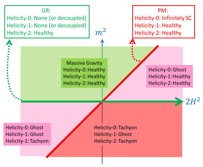
A summary of the different bounds is provided below as well as in Figure 4*:
 : Helicity-1 modes are ghost, helicity-2 and -0 are tachyonic, sick theory
 : General Relativity: two healthy (helicity-2) degrees of freedom, healthy theory,
 : One “Higuchi ghost” (helicity-0 mode) and four healthy degrees of freedom
(helicity-2 and -1 modes), sick theory,
: One “Higuchi ghost” (helicity-0 mode) and four healthy degrees of freedom
(helicity-2 and -1 modes), sick theory,
 : Partially Massless Gravity: Four healthy degrees (helicity-2 and -1 modes),
and one infinitely strongly coupled dof (helicity-0 mode), sick theory,
: Partially Massless Gravity: Four healthy degrees (helicity-2 and -1 modes),
and one infinitely strongly coupled dof (helicity-0 mode), sick theory,
 : Massive Gravity on dS: Five healthy degrees of freedom, healthy theory.
 corresponding
to GR.
corresponding
to GR.Massless and decoupling limit
- As one can see from Figure 4*, in the case where
 (corresponding to massive gravity
on AdS), one can take the massless limit
(corresponding to massive gravity
on AdS), one can take the massless limit  while keeping the AdS length scale fixed in
that limit. In that limit, the helicity-0 mode decouples from external matter sources and there
is no vDVZ discontinuity. Notice however that the helicity-0 mode is nevertheless still strongly
coupled at a low energy scale.
while keeping the AdS length scale fixed in
that limit. In that limit, the helicity-0 mode decouples from external matter sources and there
is no vDVZ discontinuity. Notice however that the helicity-0 mode is nevertheless still strongly
coupled at a low energy scale.
When considering the decoupling limit
 ,
,  of massive gravity on AdS, we
have the choice on how we treat the scale
of massive gravity on AdS, we
have the choice on how we treat the scale  in that limit. Keeping the AdS length scale
fixed in that limit could lead to an interesting phenomenology in its own right, but is yet to be
explored in depth.
in that limit. Keeping the AdS length scale
fixed in that limit could lead to an interesting phenomenology in its own right, but is yet to be
explored in depth.
- In the dS case, the Higuchi forbidden region prevents us from taking the massless limit while
keeping the scale
 fixed. As a result, the massless limit is only consistent if
  simultaneously as
  and we thus recover the vDVZ discontinuity at the linear level in
that limit.
and we thus recover the vDVZ discontinuity at the linear level in
that limit.
When considering the decoupling limit
 ,
,  of massive gravity on dS, we
also have to send
of massive gravity on dS, we
also have to send  . If
. If  in that limit, we then recover the same decoupling
limit as for massive gravity on Minkowski, and all the results of Section 8.3 apply. The case of
interest is thus when the ratio
in that limit, we then recover the same decoupling
limit as for massive gravity on Minkowski, and all the results of Section 8.3 apply. The case of
interest is thus when the ratio  remains fixed in the decoupling limit.
Decoupling limit
When taking the decoupling limit of massive gravity on dS, there are two additional contributions to take into account:
- First, as mentioned in Section 8.3.5, care needs to be applied to properly identify the helicity-0 mode
on a curved background. In the case of (A)dS, the formalism was provided in Ref. [154*] by embedding
a
 -dimensional de Sitter spacetime into a flat
  -dimensional spacetime where
the standard Stückelberg trick could be applied. As a result the ‘covariant’ fluctuation
defined in (2.80*) and used in (8.59*) needs to be generalized to (see Ref. [154*] for details)
Any corrections in the third line vanish in the decoupling limit and can thus be ignored, but the
corrections of order
-dimensional spacetime where
the standard Stückelberg trick could be applied. As a result the ‘covariant’ fluctuation
defined in (2.80*) and used in (8.59*) needs to be generalized to (see Ref. [154*] for details)
Any corrections in the third line vanish in the decoupling limit and can thus be ignored, but the
corrections of order  in the second line lead to new non-trivial contributions.
- Second, as already encountered at the linearized level, what were total derivatives in Minkowski (for
instance the combination
![2 2 [Π ] − [Π ]](article1651x.gif) ), now lead to new contributions on de Sitter. After integration
by parts,
), now lead to new contributions on de Sitter. After integration
by parts, ![m −2([Π2] − [Π]2) = m −2Rμν∂ μπ∂νπ = 12H2 ∕m2 (∂π)2](article1652x.gif) . This was the origin of the new
kinetic structure for massive gravity on de Sitter and will have further effects in the decoupling limit
when considering similar contributions from
. This was the origin of the new
kinetic structure for massive gravity on de Sitter and will have further effects in the decoupling limit
when considering similar contributions from  , where
  are defined in (6.12*, 6.13*) or
more explicitly in (6.17*, 6.18*).
are defined in (6.12*, 6.13*) or
more explicitly in (6.17*, 6.18*).
Taking these two effects into account, we obtain the full decoupling limit for massive gravity on de Sitter,
where![5 (dS) (0) H2- ∑ --λn--- (n) ℒ Λ3 = ℒΛ3 + m2 Λ3(n−1)ℒ (Gal)[π], (8.66 ) n=2 3](article1655x.gif)
 is the full Lagrangian obtained in the decoupling limit in Minkowski and given in (8.52*), and
 are the Galileon Lagrangians as encountered previously. Notice that while the ratio
  remains fixed,this decoupling limit is taken with
  , so all the fields in (8.66*) live
on a Minkowski metric. The constant coefficients
, so all the fields in (8.66*) live
on a Minkowski metric. The constant coefficients  depend on the free parameters of the
ghost-free theory of massive gravity, for the theory (6.3*) with
depend on the free parameters of the
ghost-free theory of massive gravity, for the theory (6.3*) with  and
and  , we have
At this point we may perform the same field redefinition (8.39*) as in flat space and obtain the following
semi-diagonalized decoupling limit,
where the contributions from the helicity-1 modes are the same as the ones provided in (8.52*), and the
new coefficients
, we have
At this point we may perform the same field redefinition (8.39*) as in flat space and obtain the following
semi-diagonalized decoupling limit,
where the contributions from the helicity-1 modes are the same as the ones provided in (8.52*), and the
new coefficients 
![dS) 1 μν αβ α3 + 4α4 μν (3) ∑ 5 &tidle;cn (n) ℒΛ3 = − -h ˆℰμν hαβ +------9--h Xμν + --3(n−-2)ℒ (Gal)[π ] (8.68 ) 4 8Λ 3 n=2Λ 3 + Contributions from the helicity-1 modes,](article1664x.gif)
 cancel identically for
  ,
,  and
and
 , as pointed out in [154*], and the same result holds for bi-gravity as pointed
out in [301*]. Interestingly, for these specific parameters, the helicity-0 loses its kinetic term,
and any self-mixing as well as any mixing with the helicity-2 mode. Nevertheless, the mixing
between the helicity-1 and -0 mode as presented in (8.52*) are still alive. There are no choices of
parameters which would allow to remove the mixing with the helicity-1 mode and as a result, the
helicity-0 mode generically reappears through that mixing. The loss of its kinetic term implies
that the field is infinitely strongly coupled on a configuration with zero vev for the helicity-1
mode and is thus an ill-defined theory. This was confirmed in various independent studies, see
Refs. [185*, 147*].
, as pointed out in [154*], and the same result holds for bi-gravity as pointed
out in [301*]. Interestingly, for these specific parameters, the helicity-0 loses its kinetic term,
and any self-mixing as well as any mixing with the helicity-2 mode. Nevertheless, the mixing
between the helicity-1 and -0 mode as presented in (8.52*) are still alive. There are no choices of
parameters which would allow to remove the mixing with the helicity-1 mode and as a result, the
helicity-0 mode generically reappears through that mixing. The loss of its kinetic term implies
that the field is infinitely strongly coupled on a configuration with zero vev for the helicity-1
mode and is thus an ill-defined theory. This was confirmed in various independent studies, see
Refs. [185*, 147*].
8.4  -decoupling limit of bi-gravity
We now proceed to derive the  -decoupling limit of bi-gravity, and we will see how to recover the
decoupling limit about any reference metric (including Minkowski and de Sitter) as special cases. As already
seen in Section 8.3.4, the full DL is better formulated in the vielbein language, even though in that case
Stückelberg fields ought to be introduced for the broken diff and the broken Lorentz. Yet,
this is a small price to pay, to keep the action in a much simpler form. We thus proceed in
the rest of this section by deriving the
-decoupling limit of bi-gravity, and we will see how to recover the
decoupling limit about any reference metric (including Minkowski and de Sitter) as special cases. As already
seen in Section 8.3.4, the full DL is better formulated in the vielbein language, even though in that case
Stückelberg fields ought to be introduced for the broken diff and the broken Lorentz. Yet,
this is a small price to pay, to keep the action in a much simpler form. We thus proceed in
the rest of this section by deriving the  -decoupling of bi-gravity and start in its vielbein
formulation. We follow the derivation and formulation presented in [224*]. As previously, we focus on
-decoupling of bi-gravity and start in its vielbein
formulation. We follow the derivation and formulation presented in [224*]. As previously, we focus on
 -spacetime dimensions, although the whole formalism is trivially generalizable to arbitrary
dimensions.
-spacetime dimensions, although the whole formalism is trivially generalizable to arbitrary
dimensions.
We start with the action (5.43*) for bi-gravity, with the interaction
where the relation between the![∫ M 2Plm2 4 √--- ∑4 ℒg,f = ---4--- d x − g αn ℒn [𝒦 [g,f]] (8.69 ) ∫ n=0 M 2Plm2 [β0 a b c d β1 a b c d = − ------𝜀abcd --e ∧ e ∧ e ∧ e + --f ∧ e ∧ e ∧ e (8.70 ) 2 4! 3! ] + β2-f a ∧ fb ∧ ec ∧ ed + β3f a ∧ f b ∧ fc ∧ ed + β4fa ∧ fb ∧ fc ∧ f d , 2!2! 3! 4!](article1673x.gif)
 ’s and the
  ’s is given in (6.28*).
We now introduce Stückelberg fields  for diffs and
  for the local Lorentz. In the
case of massive gravity, there was no ambiguity in how to perform this ‘Stückelbergization’ but in the case
of bi-gravity, one can either ‘Stückelbergize the metric
for the local Lorentz. In the
case of massive gravity, there was no ambiguity in how to perform this ‘Stückelbergization’ but in the case
of bi-gravity, one can either ‘Stückelbergize the metric  or the metric
  . In other words the
broken diffs and local Lorentz symmetries can be restored by performing either one of the two replacements
in (8.69*),
. In other words the
broken diffs and local Lorentz symmetries can be restored by performing either one of the two replacements
in (8.69*),


Since we are interested in the decoupling limit, we now perform the following splits, (see Ref. [419] for more details),
and perform the scaling or decoupling limit, while keeping Before performing any change of variables (any diagonalization), in addition to the kinetic term for quadratic


 ,
,  and
and  , there are three contributions to the decoupling limit of
bi-gravity:
, there are three contributions to the decoupling limit of
bi-gravity:
- ❶
- Mixing of the helicity-0 mode with the helicity-1 mode
 , as derived in (8.52*),
- ❷
- Mixing of the helicity-0 mode with the helicity-2 mode
 , as derived in (8.40*),
- ❸
- Mixing of the helicity-0 mode with the new helicity-2 mode
 ,
,
noticing that before field redefinitions, the helicity-0 mode do not self-interact (their self-interactions are constructed so as to be total derivatives).
As already explained in Section 8.3.6, the first contribution ❶ arising from the mixing between the
helicity-0 and -1 modes is the same (in the decoupling limit) as what was obtained in Minkowski (and
is independent of the coefficients  or
or  ). This implies that the can be directly read
of from the three last lines of (8.52*). These contributions are the most complicated parts of
the decoupling limit but remained unaffected by the dynamics of
). This implies that the can be directly read
of from the three last lines of (8.52*). These contributions are the most complicated parts of
the decoupling limit but remained unaffected by the dynamics of  , i.e., unaffected by the
bi-gravity nature of the theory. This statement simply follows from scaling considerations. In
the decoupling limit there cannot be any mixing between the helicity-1 and neither of the two
helicity-2 modes. As a result, the helicity-1 modes only mix with themselves and the helicity-0
mode. Hence, in the scaling limit (8.74*, 8.75*) the helicity-1 decouples from the massless spin-2
field.
, i.e., unaffected by the
bi-gravity nature of the theory. This statement simply follows from scaling considerations. In
the decoupling limit there cannot be any mixing between the helicity-1 and neither of the two
helicity-2 modes. As a result, the helicity-1 modes only mix with themselves and the helicity-0
mode. Hence, in the scaling limit (8.74*, 8.75*) the helicity-1 decouples from the massless spin-2
field.
Furthermore, the first line of (8.52*) which corresponds to the dynamics of  and the helicity-0 mode
is also unaffected by the bi-gravity nature of the theory. Hence, the second contribution ❷ is the also the
same as previously derived. As a result, the only new ingredient in bi-gravity is the mixing ❸
between the helicity-0 mode and the second helicity-2 mode
and the helicity-0 mode
is also unaffected by the bi-gravity nature of the theory. Hence, the second contribution ❷ is the also the
same as previously derived. As a result, the only new ingredient in bi-gravity is the mixing ❸
between the helicity-0 mode and the second helicity-2 mode  , given by a fixing of the form
 .
.
Unsurprisingly, these new contributions have the same form as ❷, with three distinctions: First the way
the coefficients enter in the expressions get modified ever so slightly ( and
and  ). Second,
in the mass term the space-time index for
). Second,
in the mass term the space-time index for  ought to dressed with the Stückelberg field,

 (which enters in the mass term) is now a function of
the ‘Stückelbergized’ coordinates
(which enters in the mass term) is now a function of
the ‘Stückelbergized’ coordinates  , which in the decoupling limit means that for the mass term
These two effects do not need to be taken into account for the
, which in the decoupling limit means that for the mass term
These two effects do not need to be taken into account for the ![a a μ μ 3 a v b = vb[x + ∂ π∕Λ 3] ≡ vb[&tidle;x]. (8.77 )](article1703x.gif)
 that enters in its standard curvature
term as it is Lorentz and diff invariant.
that enters in its standard curvature
term as it is Lorentz and diff invariant.
Taking these three considerations into account, one obtains the decoupling limit for bi-gravity,
with![ℒ (bi−gravity) = ℒ (0)− 1vμν[x]ˆℰαβvαβ[x] (8.78 ) Λ3 Λ3 4 μν 1 M ( Πν ) ∑3 &tidle;β − ----Plvμβ[&tidle;x] δνβ + -β3- -3n(+n1−1)Xμ(nν)[Π], 2 Mf Λ3 n=0 Λ3](article1705x.gif)
 . Modulo the non-trivial dependence on the coordinate
  ,
this is a remarkable simple decoupling limit for bi-gravity. Out of this decoupling limit we can re-derive all
the DL found previously very elegantly.
,
this is a remarkable simple decoupling limit for bi-gravity. Out of this decoupling limit we can re-derive all
the DL found previously very elegantly.
Notice as well the presence of a tadpole for  if
if  . When this tadpole vanishes (as well as the
one for
. When this tadpole vanishes (as well as the
one for  ), one can further take the limit
  keeping all the other
  ’s fixed as well as
  ,
and recover straight away the decoupling limit of massive gravity on Minkowski found in (8.52*), with a free
and fully decoupled massless spin-2 field.
,
and recover straight away the decoupling limit of massive gravity on Minkowski found in (8.52*), with a free
and fully decoupled massless spin-2 field.
In the presence of a cosmological constant for both metrics (and thus a tadpole in this framework), we
can also take the limit  and recover straight away the decoupling limit of massive gravity on
(A)dS, as obtained in (8.66*).
and recover straight away the decoupling limit of massive gravity on
(A)dS, as obtained in (8.66*).
This illustrates the strength of this generic decoupling limit for bi-gravity (8.78*). In principle we could
even go further and derive the decoupling limit of massive gravity on an arbitrary reference metric as
performed in [224*]. To obtain a general reference metric we first need to add an external source for  that generates a background for
  . The reference metric is thus expressed in the local
inertial frame as
. The reference metric is thus expressed in the local
inertial frame as
 looks like a perturbation away from Minkowski is related to the fact that the
curvature needs to scale as
looks like a perturbation away from Minkowski is related to the fact that the
curvature needs to scale as  in the decoupling limit in order to avoid the issues previously mentioned in
the discussion of Section 8.2.3.
in the decoupling limit in order to avoid the issues previously mentioned in
the discussion of Section 8.2.3.
We can then perform the scaling limit  , while keeping the
  ’s and the scale
 fixed as well as the field
  and the fixed tensor
  . The decoupling limit is then
simply given by
. The decoupling limit is then
simply given by
![( ν) 3 ℒ(¯U)= ℒ(0)− 1¯U μβ[&tidle;x ] δν + Π-β ∑ --&tidle;βn+1-X (n)[Π ] (8.81 ) Λ3 Λ3 2 β Λ33 Λ3 (n− 1) μν n=0 3 − 1vμνℰˆαβv , 4 μν αβ](article1725x.gif)
 fully decouples from the rest of the massive gravity sector on the
first line which carries the other helicity-2 field as well as the helicity-1 and -0 modes. Notice
that the general metric
fully decouples from the rest of the massive gravity sector on the
first line which carries the other helicity-2 field as well as the helicity-1 and -0 modes. Notice
that the general metric  has only an effect on the helicity-0 self-interactions, through the
second term on the first line of (8.81*) (just as observed for the decoupling limit on AdS). These
new interactions are ghost-free and look like Galileons for conformally flat
has only an effect on the helicity-0 self-interactions, through the
second term on the first line of (8.81*) (just as observed for the decoupling limit on AdS). These
new interactions are ghost-free and look like Galileons for conformally flat  , with
 constant, but not in general. In particular, the interactions found in (8.81*) would not be
the covariant Galileons found in [166, 161, 157*] (nor the ones found in [237*]) for a generic
metric.
constant, but not in general. In particular, the interactions found in (8.81*) would not be
the covariant Galileons found in [166, 161, 157*] (nor the ones found in [237*]) for a generic
metric.
 |
 |
 |
Living Rev. Relativity, 17 (2014), 7, doi:10.12942/lrr-2014-7, URL (accessed <date>): http://www.livingreviews.org/lrr-2014-7.
 This work is licensed under a Creative Commons License.
© The author(s), except where otherwise noted.
This work is licensed under a Creative Commons License.
© The author(s), except where otherwise noted.